Chapter 8: Alignment of 3 Centers of Curvature
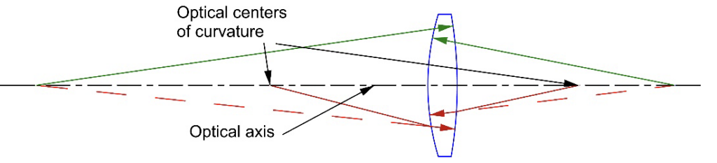
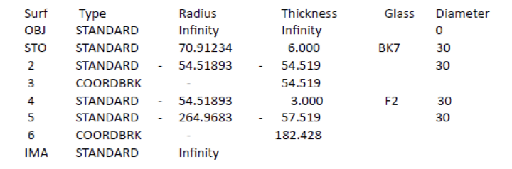
A convenient and concrete example of aligning three centers of curvature is the cementing of the doublet we used in the optical axis example in Chapter 5, the details of which are reproduced below.
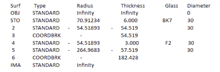
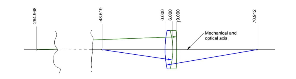
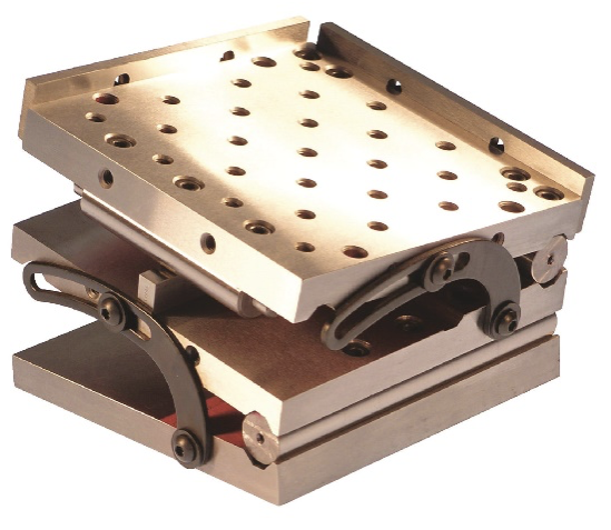
Fig. 1 Doublet used as an example of aligning three centers of curvature
The goal is to get all three centers of curvature on the same line to some tolerance dictated by the desired lens system performance. When alignment and centering is done in practice the meniscus element is placed on a seat with the concave surface facing up so that when a drop of cement is added it is contained within the concave well. We have already been over the details of aligning the optical axis, or two centers of curvature, of the meniscus to a seat in Chapter 7.
As seen in Fig. 1, the task now is to align the upper convex surface of the positive element so that its center of curvature lies on the optical axis of the meniscus. The interface between the two lens elements takes care of itself as the cement acts as a lubricant between the interface surfaces. The cement is worked out to a thin uniform thickness by pressing down and gently sliding the positive element around on the meniscus. Once the cement is thin enough that there is a drag resisting the sliding the positive element is centered and the cement cured.
Because the surface facing the alignment sensor and its objective is convex, the objective must have a working distance of more than the radius of the upper surface, or roughly 71 mm in this case. Unless the diameter of the lens being cemented is quite small, the convex surface will be longer than most commercially available microscope objectives. Autocollimator type centering sensors come with a variety of working distance objectives and autostigmatic microscopes can be fitted with simple doublet objectives to get the required working distance.
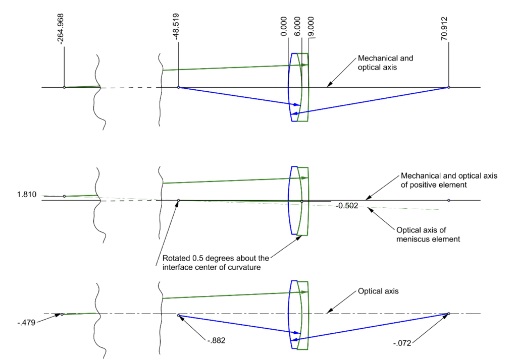
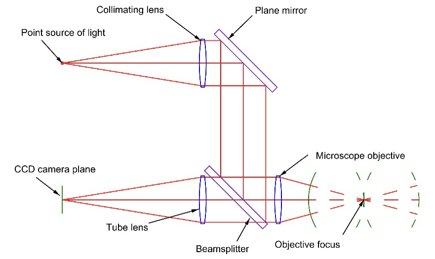
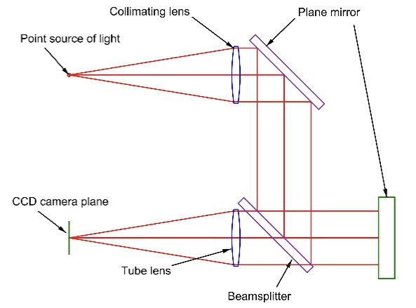
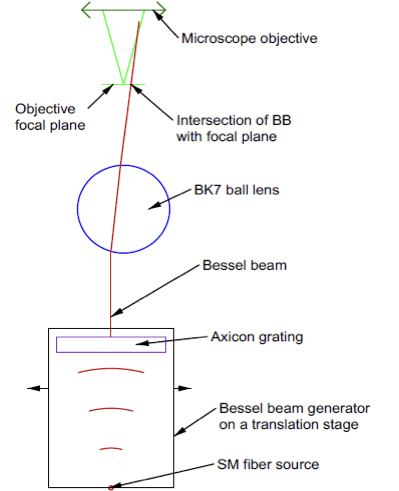
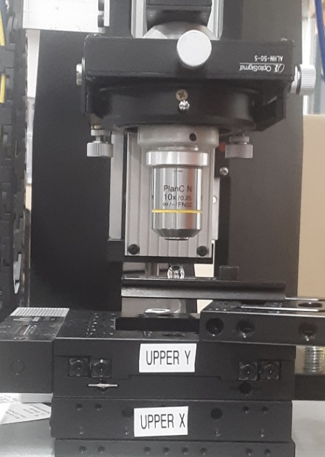
While using an objective with a long enough efl will almost always reach the center of curvature, there is a loss in sensitivity to alignment due to the increase in the focal length of the objective. For cementing doublets this is probably not an issue because the longer the radius, the weaker the lens and the less sensitive the lens is to alignment. There are cases where the doublet has a large diameter and is relatively fast where alignment can be an issue so there is a need for greater sensitivity. There are other occasions where there is physical interference, and a long working distance is needed to reach the center of curvature. In these cases, it is possible to add a 1 to 1 relay in front of the objective that has sufficient sensitivity. An example of such a relay for use with an autostigmatic microscope is shown in Fig. 2. This makes an aesthetically ungainly instrument but achieves the purpose of no loss of sensitivity.
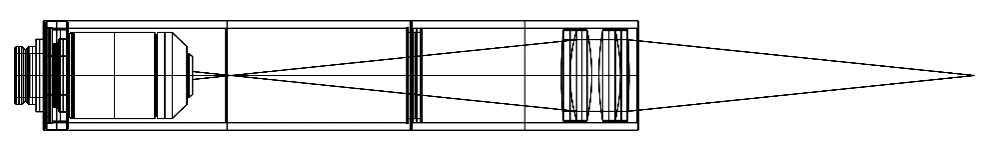
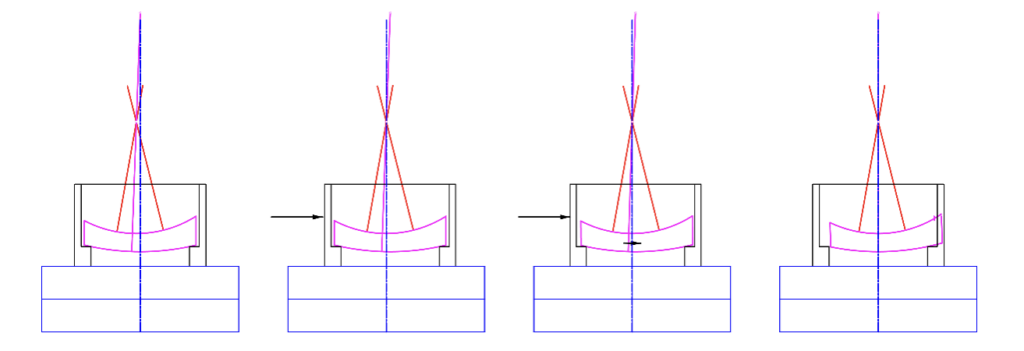
Fig. 2 Long working distance objective with same lateral sensitivity as the microscope objective
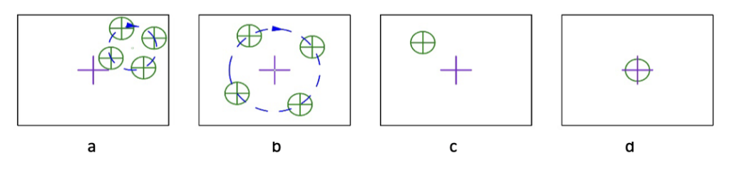
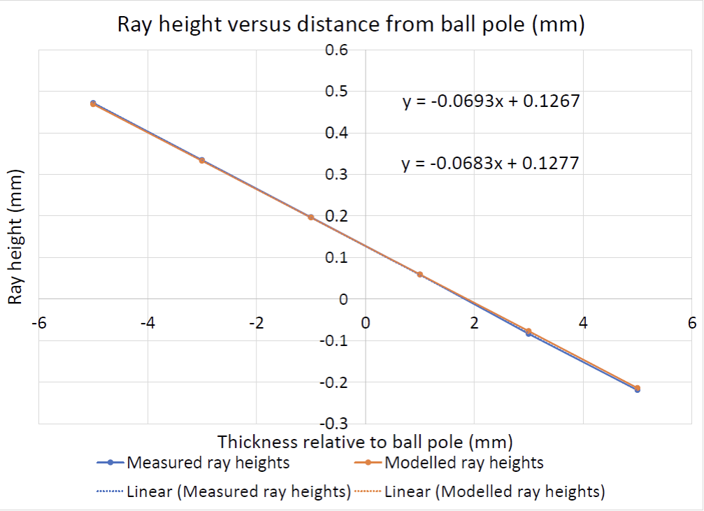
Going back to our example, assuming we use an objective with a 100 mm efl to reach the center of curvature of the upper surface, we have a situation as in Fig. 3. The 0.5° (0.0087 radian) tilt of the positive element moves its center of curvature 1.042 mm off the axis of the meniscus. Since almost any optical sensor can detect a µm decenter and there is a 2x magnification of the displacement due to reflection, the center of curvature location is easily measurable to 1 second of arc, better than any but the most stringent centering requirement.
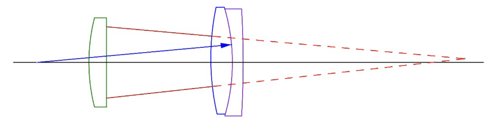
Fig. 3 Light from a 100 mm efl objective reflecting from the 0.5° tilted positive doublet element showing the displaced center of curvature of the convex surface rotated about the interface surface
Figure 3 shows the mechanical implications of being able to center to 1 second of arc. From similar triangles, the positive element is about 1/3 of the distance from the objective to the center of curvature which implies that the edge of a perfectly centered element will be aligned to a perfect meniscus to about 1/3 of a µm, far better than such an element is realistically edged.
What I am trying to illustrate here is that aside from very small (cell phone camera and endoscope lenses) and very large lenses, relying on mechanical tolerances of the edges of elements may not be the optimum approach where precision centering is needed. Optical centers of curvature are the critical features for alignment, not mechanical interfaces at the edges. The peripheral mechanical interfaces should be designed to allow for the adjustment of the centers of curvature, but these interfaces should not be the features that define the alignment when high precision is needed.
As an example, some doublets are centered and cemented using a “V” block to align the edges of the elements. Assume we want to align our example doublet to 3 minutes of arc or about 1 milliradian, a typical centering tolerance for good but not precision centering. This means that the 2 elements must be edged within 50 µm of the same diameter to meet this tolerance assuming no other errors in the centering process. If there is any wedge in either of the elements there will be additional errors.
I think the idea of the use of optical versus mechanical features for alignment goes beyond the optical elements themselves. Consider the typical rotary table centering device. It uses a mechanical axis of rotation to define the reference axis to which we want to align our optical elements. In one sense this is an ideal method of centering as we have previously illustrated; if the transmitted or reflected image from an optical surface moves it does not lie on the axis of the rotary table, full stop. However, we have optical centering sensors that detect motion of an image to a fraction of a µm. That means the runout of the table must be less than a µm to make use of the full sensitivity of the sensor.
In addition, the tilt or wobble, of the table must be small and the further the optic being centered is above the table the worse the effect may be. Assume our table has a 1 second of arc (5 µradian) tilt and the optic we are aligning is 100 mm above the table. As the table rotates the mechanical vertex of the element will translate ± 0.5 µm and if our sensor could see a mark at the vertex, it would be seen to move 1 µm TIR (total indicator reading, a terminology from mechanical touch indicators).
However, our optical sensor is not viewing the vertex of the element but rather the center of curvature. In the case of our example doublet we have the situation in Fig. 4 where the center of curvature of the upper surface lies near the rotary table surface.
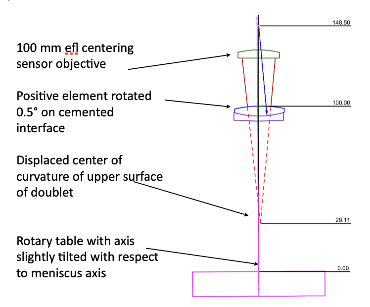
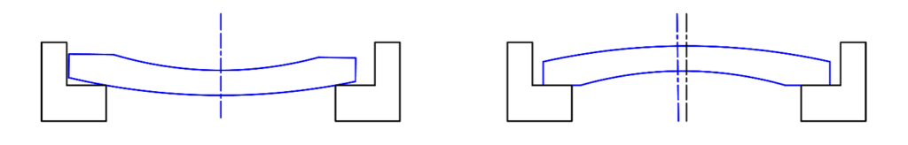
Fig. 4 Misaligned doublet on rotary table having a tilt error
Since the center of curvature lies near the table and we assume that the tilt in the table occurs near the table surface, the motion of the center of curvature is reduced by the ratio of 29/100. The reverse is true of the interface surface, its CoC moves more by the ratio 148.5/100 and the CoC of the lower surface of the meniscus by 356/100.
To minimize the errors in rotary tables they almost always are equipped with adjustment screws to remove the tilt and decenter that rotate in synchronism with the table. Errors of a higher frequency than once per revolution cannot be removed by these adjustments, however. The precision of alignment using a rotary bearing as the reference axis is never better than the quality of the bearing.
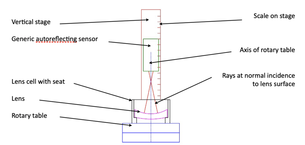
If the quality of the rotary bearing limits the precision of centering, what if the lens remained stationary? Then the quality of the vertical slide becomes the limiting factor because you must rely on its precision to move the sensing unit from one center of curvature to the other to establish the axis of the lens. This is not a new idea and was proposed in a paper1 a few years ago. The paper points out the advantage of this method. Assuming a sufficiently high precision vertical stage, the method is much faster than using a rotary table because there is immediate feedback of the result of making a centering adjustment.
When a rotary table is used you make an adjustment and then rotate the table to see if the adjustment has improved the centering. If the lens is stationary, you are making the adjustment to drive the reflected image to a particular position in the sensor coordinate system and can directly see how fast and far the reflected spot is moving without worrying about rotating the table. The paper estimates that eliminating the rotary table would speed up the alignment process by a factor of 5-6. To the best of my knowledge a product has never been brought to market based on this method. This may indicate that the method is not easy to implement in this form despite its apparent advantages.
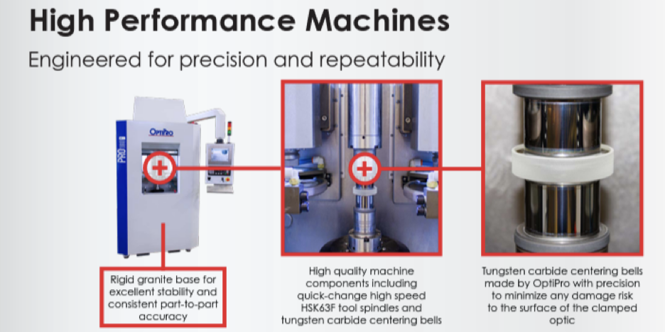
The idea has merit, however. It depends on how the vertical slide is designed and implemented. Think of the possibility of using the vertical ram (the arm of the machine the probe is attached to) of a coordinate measuring machine (CMM) as the vertical slide. Even relatively inexpensive CMMs read out the probe location to ± 1 µm. This does not mean the probe moves with µm straightness, but that the calibration method and software tell you where the probe is in 3 degrees of freedom (DOF) to on the order of ± 1 µm plus a factor for the distance moved. Compared to the price of a precision centering device with a rotary table, a CMM with an optical sensor may be a cost effective method when it is balanced with productivity improvement. You only purchase the hardware once; you pay for labor every day.
Using a CMM for centering2 still means you must raise and lower the ram to go from one CoC to the other. The adjustment at each CoC is much faster than with the rotary table it but will still take more than one look at each CoC to make sure the best alignment is achieved. Further, the method still depends on precision mechanical motion and calibration. What if centering to remove tilt and decenter could be done without having to move any part of the centering measuring device? What if the only adjustments were the 4 that adjust tilt in 2 DOF and decenter in 2 DOF. The method would be faster and more precise.
I have hinted at the method in Chapter 5 where we define the optical axis of a multi-element system as a line in space representing a single transmitted ray that is unchanged in location or direction when the lens is inserted in the ray path. In the next Chapter I will talk about how to generate a single ray that is useful for aligning optical systems in general but specially for centering of lenses to an optical reference axis.
1 J. Heinisch, F. Hahne, P. Langehanenberg, “Rotation-free centration measurement for fast and flexible inspection of optical lens systems,” Proc. SPIE 11175, 111751B (2019)
2 https://www.youtube.com/watch?v=FoeMAT8PfjU