New Product Launch
Optical Perspectives Group proudly introduces PSM Align
Revolutionary Python-Based Software for Point Source Microscope
Now Standard on All PSM Units

Author: csadmin

What is an Autostigmatic Microscope (ASM) and the Origin of the Point Source Microscope (PSM)

When most people think of a microscope it is one that works in transmission with the light source on one side of the sample and the microscope objective and eyepiece on the other. An autostigmatic microscope (ASM) works in reflection, just like an autocollimator, so the light source is in the microscope body, and is almost always introduced via a beamsplitter close to the objective but between objective and eyepiece as shown in Fig.1.
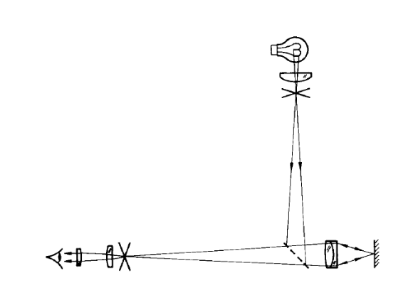
Fig. 1 An autostigmatic microscope (from Steel[1])

An ordinary reflecting microscope such as one used to examine opaque samples uses an extended light source that is imaged on the entrance pupil of the objective so that the light is made to uniformly flood the sample over the microscope field of view. An autostigmatic microscope is different in this respect in that a crosshair or pinhole source of light is placed conjugate, via the beamsplitter, to the eyepiece object plane. This means that an image of the crosshair or pinhole will be in focus at the focus of the microscope objective. In some very simple cases, the coiled filament of the light bulb making up the source is conjugate to the eyepiece object place so that when the microscope is focused on a surface the filament is in good focus viewed through the eyepiece.

This rather long description of an ASM is necessary because there are almost no literature references to them yet they are a staple in almost every optics shop for use in measuring test plate, or lens surface, radii of curvature. The only literature reference I have found is a paper1 by W. H. Steel titled “The Autostigmatic Microscope”, although he cites a reference to C. V. Drysdale2 in 1900, “ON A SIMPLE DIRECT METHOD OF DETERMINING THE CURVATURES OF SMALL LENSES”. Drysdale started the Technical Optics Department at Northampton Institute in that same year, so it is clear ASMs have been around for over a century.

Going back to Steel, his paper describing an ASM was probably written for the same reason as this paper, his audience had very little idea what an ASM was and what it was used for. His audience happened to be optometrists because he was working at CSIRO, the Australian version of the US NIST, on a job to measure the radii of curvature of contact lenses back in 1983. In the abstract to the paper he stated “The autostigmatic microscope is an instrument for measuring the line-of-sight distance to areflecting surface and is used chiefly to measure the radii of lens surfaces.”, and goes on to say the ASM is an analog of an autocollimator that focuses at a finite distance rather than infinity.

The one other place I have seen mention of an ASM is in Warren Smith’s book, “Modern Optical Engineering” toward the very end where he calls it an autocollimating microscope3 and ascribes to it the same use as Steel. The implication in Malacara’s Optical Shop Testing4 is that one would obviously use an ASM in many cases of testing but ASMs are never mentioned explicitly.

How the ASM works

Before going further we should explain how the ASM works in the two modes used to measure radii. The principles are most easily explained by considering the light source as a pinhole conjugate with the object plane of the eyepiece. In this case, an image of the pinhole will appear at the objective focus and be smaller than the pinhole source by the magnification of the objective. If the pinhole source was 50 μm in diameter, it would appear as 5 μm in diameter at the focus of a 10x objective. Also note, as in Fig. 1, microscopes in the time frame of Steel’s paper used finite conjugate objectives so the objective was the only optical element with power in the microscope. This is a perfect example of a stigmatic optical system, one that images a point of light in the object plane into a perfect point in the image plane.5

If the ASM was focused on a specular surface as in Fig. 2, the light coming from the top part of the objective would reflect off the surface and re-enter the objective at the bottom, and vice versa. This is the so called Cat’s eye, or retroreflection, focus. Notice that the surface does not have to be normal to the optical axis of the objective, the reflected light will always return to the pinhole source on the other side of the meridional plane from which it started out. The reflecting surface can be tilted from normal until none of the reflected light makes its way back into the objective, but whatever light does make it into the objective will always focus on the source pinhole.
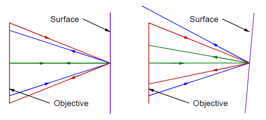
Fig. 2 Cat’s eye reflection with surface normal to optical axis of objective (left) and with surface tilted (right)

As a consequence of this retroreflection behavior, the reflected light passing through the beamsplitter to the eyepiece will always focus in the same place laterally in the eyepiece object plane, and this place is exactly conjugate to the pinhole light source. If the objective is not in good focus on the surface the reflected spot will be out of focus but always centered in the same location independent of the tilt of the surface. At best focus the image in the eyepiece object plane will be exactly the same size as the pinhole in the source. Notice that this is the same type of behavior as putting a cube corner reflector in front of an autocollimator, the reflected light spot is stationary even when the cube corner is no longer square with the axis of the autocollimator.

The other location where reflected light returns to the ASM is if the focus of the objective is at the center of curvature of a spherical surface as in Fig. 3a where the objective is focused on the center of the ball, here used as a convex mirror. Light rays exiting the objective follow normals to the surface of the spherical ball, and light is reflected back along the normals into the objective. If, however, the focus of the objective is slightly to the side of the center of curvature as in Fig. 3b, the return light will focus on the opposite side of the center of curvature. This makes the ASM very sensitive to alignment with the center of curvature of a spherical surface. Obviously, just as in the case of the Cat’s eye reflection the return spot of light will be out of focus if the objective focus is not coincident with the center of curvature along the line of sight to the surface.
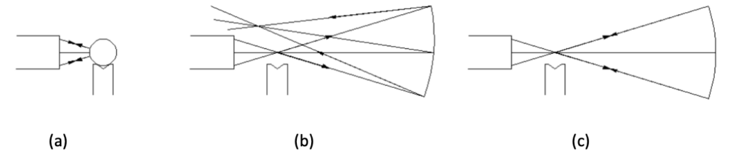
Fig. 3 Objective focused at the center (of curvature) of a ball, or convex mirror (a), focused near the center of curvature of a concave sphere (b) and focused precisely at the center of curvature (c)

With this background it is now easy to see how an ASM can be used to measure the radius of curvature of a lens or mirror surface. First focus the ASM on the surface near its center and the Cat’s eye reflection will appear in good focus when the ASM is precisely focused on the surface. Adjust the cross hairs or other reference in the eyepiece on the return spot as this reflected image is at the conjugate of the light source, and on the optical axis of the ASM.

Then move the ASM to focus at the center of curvature of the surface by aiming the ASM roughly at the center of the surface and moving in 3 degrees of translation until the return reflected spot lies centered on the eyepiece crosshairs or reference. The ASM is now precisely located at the center of curvature in 3 degrees of freedom. Note the position of the ASM base on a rule or straightedge lying between the ASM and surface. Move the ASM along the straightedge until the Cat’s eye reflection is again in focus and note the scale reading. The difference in the 2 readings as shown in Fig. 4 is the radius of curvature of the surface. Note that by moving along a straightedge from a position where the ASM was centered at the center of curvature means that the ASM is moving along a normal to the sphere and a true reading of the radius of curvature will be achieved.
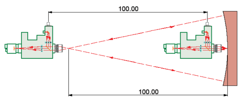
Fig. 4 Use of an ASM to measure the radius of curvature of a concave mirror

Notice also that this method works equally well for convex surfaces as long as the objective has a long enough working distance to accommodate the radius of the surface. Another issue to keep in mind is that the laws of physics still apply to radius measurement. If the surface being measured has a small diameter relative to its radius of curvature there will be difficulty finding best focus due to the slow f/# of the light cone. On the Cat’s eye side, a higher magnification objective permits greater sensitivity to focus but at the center of curvature may throw away too much light beyond the edge of the surface. In general, use a low magnification objective like 5x for slow surfaces and a 10 or 20x objective for fast surfaces.

My introduction to autostigmatic microscopes

My first job after getting out of school with a MA in Physics and no formal optics education was at Eastman Kodak Company. Virtually the first thing they had me do was measuring the radius of curvature of test plates, the master surfaces against which lens surfaces would be checked using Newton ring interference. The measurement was done with an ASM whose make I forget but it could have been one from Gaertner Scientific6, a company that still sells all the parts needed to make an ASM. Another project at Kodak got me into issues of aligning one optic to another but the idea of using an ASM as an alignment device did not click in my mind.

From Kodak I went to Itek Corporation (now a part of Goodrich) in Lexington, MA. One of my jobs there was to adjust the 6 cameras in the S-190 survey instrument7, flown on Skylab in the summer of 1973, for matched distortion and magnification. Each camera operated in a different spectral band and the idea was to be able to overlay the 70 mm format negatives from the different cameras and have details in the film match up to +/- 1 μm. This meant each nominally 150 mm focal length camera had to beadjusted to have nearly identical field heights at the edges of the field even though some of the spectral bands were outside the visible spectrum into the IR.
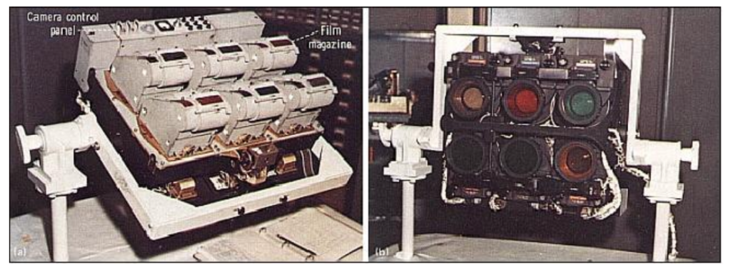
Fig. 5 S-190A Multispectral Photographic Camera System

We used a nodal slide lens bench to do the measurement and projected a collimated beam of white light from a pinhole source into each of the cameras. The point images in the camera focal planes were detected with a microscope that had a quad cell photo detector in the eyepiece object plane. There was a beamsplitter so that the images could be viewed either visually or electronically. The visual image allowed us to get things aligned initially but the data were taken for all 6 cameras using the electronic quad cell so all the distortion and magnification data were all treated the same. This use of a microscope with an electronic detector put another piece of the ultimate ASM design in the back of my mind.

From Itek I went on to work at Frank Cooke, Inc. in central Massachusetts and learned how optics were really made instead of just testing them. One of the items made there was a hyper-hemispherical glass dome about 180 mm in diameter and 6 mm thick. There was a reasonably tight spec on the concentricity of the inner and outer surfaces of the dome, that is, the centers of curvature of the 2 surfaces were supposed to be within 50 μm of each other in all 3 degrees of freedom.

The person in charge of testing at Cooke’s was Raymond Boyd who had formerly worked for American Optical in Southbridge, MA. To test for concentricity, Ray effectively made an ASM by inserting a piece of optical fiber in a filar eyepiece much as in Fig. 6.
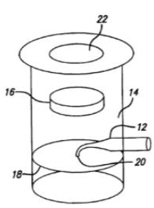
Fig. 6 Illustration from US Patent 6,924,897 showing an eyepiece with a fiber point light source. 12 is the fiber preform, 20 the drawn out tip, 18 the eyepiece focal plane and 16 the eyepiece lens

Ray had worked with Elias Snitzer, one of the early inventors of fiber optics at American Optical, and had access to fiber optic pre-forms that were about 3 mm in diameter. Ray would use an alcohol flame to draw the preform out into a small diameter fiber and bend the tip 90 degrees to make a rudimentary point source. He used a microscope illuminator focused on the large end of the preform as the light source. When the fiber tip was at the centers of curvature of the dome, point images were returned from both surfaces and the distance separating them could easily be measured with the filar scale in the eyepiece focal plane.

This simple optical device could do in minutes what would otherwise be a complex mechanical metrology problem requiring a good rotary bearing and several contact measurements along with some math to determine the same knowledge of the concentricity of the surfaces. We used similar fibers to test such things as fast elliptical reflectors as described in a brief paper8 I wrote after moving on to run the Optics Shop at the Optical Sciences Center at the University of Arizona.

While at Optical Sciences I found that EG&G was making an eyepiece for a radiometric instrument they sold that was almost identical to the one Ray Boyd had used at Cooke’s. EG&G used the eyepiece backwards to how we intended to use it; the tip of the fiber picked up light coming toward the eyepiece from the sample being viewed and a fiber bundle took that light to a sensitive photometer to record its value. We illuminated the end of the fiber bundle with a bright source and let the light exit the tip in the eyepiece headed out of the microscope through the objective. When the objective was focused on a specular surface the light from the fiber came back in retroreflection directly on the fiber tip in the eyepiece. This was a great, commercially available, solution to making a point source eyepiece for an ASM. Unfortunately, not many years later EG&G stopped making these eyepieces.

About this time I left the University to start a consulting company called Optical Perspectives Group, LLC along with a colleague, William P. (Bill) Kuhn. One day we got call from a local company that had designed a complex lens for a laser writer system they were making. The system had 6 lenses, some of which were rectangularly edged toroids, and a spherical mirror, all of whose centers of curvature were supposed to lie on a straight line. Our job was to come up with a method of aligning the lenses and mirror so this was the case.

We immediately recognized this was a perfect job for an ASM which we put together with Thorlabs parts and an analog CCD camera. The ASM was mounted in the chuck of a milling machine and the optical bench holding the lens elements was set on the mill table that we used as a large x-y-z stage. With this set up we were able to get to the centers of curvature of all the elements by cranking the mill table over the length of its travel. In the case of the toroidal lenses we would get back line images instead of a circular spots but the lines were just as easy to align as the spots.

Using this crude ASM and the mill we were able to align the lens system in about 4 hours and get better performance from the system than they had previously by another method that took about 2 weeks. The company was delighted, but the system needed to be assembled in a clean room environment and they could not put the mill in the clean room.

This was the beginning of the original Point Source Microscope (PSM), an ASM small and light enough to be held on the ram of a coordinate measuring machine (CMM) in place of the usual mechanical touch probe. Many advances in technology had been made over the years since the ASM put together at Cooke’s. There were affordable CCD cameras and single mode fiber light sources in the visible. Also, microscope design had changed from a finite conjugate to infinite conjugate version where the lightbetween the objective and “tube lens” was collimated. The reason for this change was that it made customizing microscopes much easier since the distance between the eyepiece and objective did not have to stay fixed. It also meant that in reflecting microscopes the beamsplitter that was necessary to introduce the light from the source no longer introduced aberrations into the converging beam of light in finite conjugate microscopes.

The initial major problem with the new PSM was there was no easy way to mark where the Cat’s eye reflection returned on the detector. Our initial solution was to place a Magic Marker dot on the analog monitor faceplate. This worked but was neither elegant nor precise. We then realized that a Shack cube, such as used in a Shack cube interferometer9, would be just what was needed to produce a reference spot of light to be the indication of where to bring the light to focus from the center of curvature of the surface we were trying to align. Fig. 7, taken from US Patent 6,924,897, shows the original PSM layout and the Shack cube (#30).
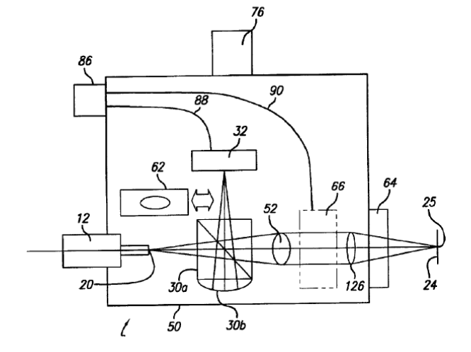
Fig. 7 Layout of the original Point Source Microscope

The Shack cube is a cube beamsplitter with plano-convex lens cemented to one side so that its center of curvature is conjugate to the tip of a single mode optical fiber (20) and the analog CCD camera. The objective is #126 and the tube lens is #52 with collimated space in between. While this design worked very well for our customer, we realized almost immediately that this was not a very smart design; once the return spot was centered behind the reference spot there was no way to center any better. This limited our centering ability to about 5 μm. At the same time useful technology was moving forward at a fast pace.

Bill looked at a combination of the short comings of this original design and advances in technology to come up with what is now sold as the PSM, and is shown schematically in Fig. 8. There are many improvements on the original but the one to address the major flaw of the first was to use a digital CCD camera coupled with National Instruments LabView software that could centroid on the return spot of light. This meant that when the Cat’s eye spot was first obtained in good focus the software could place an electronic crosshair on the video display to define the lateral zero position on the display to a fraction of a μm. Other return spots could then be located relative to the crosshair to the same precision.
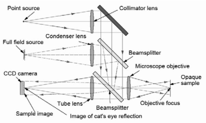
Fig. 8 A schematic diagram of the optical paths within the PSM

Going back to Fig. 8, other new features included an internal LED light source and diffuser to provide Kohler illumination for full field imaging so the PSM could be used as an ordinary video microscope as well as an autostigmatic one for alignment purposes. Where the original PSM had an external fiber source the new one has a single mode fiber pigtailed to a red laser diode. The two light sources are adjusted so the autostigmatic focus is parfocal with the full field image plane. Another feature of the laser diode light source is that it has a bright and dim mode. In the bright mode the light is bright enough to be seen under ambient lighting so that it is easy to find the return reflected light spots. However, this intensity is sufficient to saturate the camera in most cases so the dim mode is used for the electronic centroiding.

A further feature is the use of infinite conjugate optics so that when the objective is removed from the PSM it becomes an autocollimator. Thus the PSM is 3 distinct instruments in one, a video imaging microscope, an ASM and an autocollimator with an exceptionally large angular capture range.

Using the PSM for alignment

Now that the development of the PSM and the use of it to measure radii of curvature have been described, we will describe a simple but non-trivial alignment situation. Assume we want to align the optics in a 2 mirror grating spectrometer that, when aligned, looks like Fig. 9. We will assume that the 2 slits and the axis of the grating are fixed by the mechanics of the lens bench on which the optics are mounted. From a combination of the mechanical and optical drawings of the instrument we know where the centers of curvatures of the collimating mirrors should be relative to the slits and grating axis before the optical path is folded to the slits. Further, the 2 fold mirrors should be set so that light focused at the entrance slit exits in focus at the exit slit. Also assume that all 4 mirrors that will be aligned are held in mounts with 3 adjustment screws so they may be tilted in 2 directions and displaced axially in the direction of the screws by turning all 3 simultaneously.
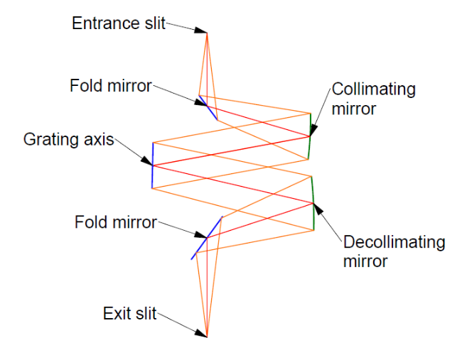
Fig. 9 A two mirror grating spectrometer in its final configuration

Fig. 10 shows where the centers of curvature of the collimating mirrors are (violet) and where they are reflected in the fold mirrors (blue) when the fold mirrors are properly aligned.
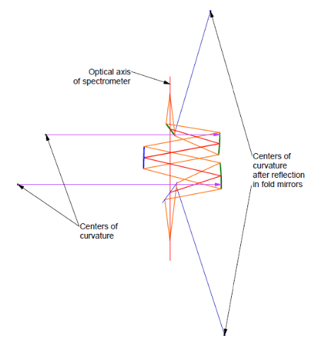
Fig. 10 The center of curvature locations of the collimating mirrors directly and as folded

To perform the alignment the optical bench on which the mirrors and grating are mounted are temporarily mechanically pinned to an alignment fixture plate into which holes have been bored at the center of curvature and slit locations. Into these holes a post is placed on the top of which is a spherical steel ball. An example of this type fixture is shown in Fig. 11 where the posts are lens mount posts and the balls sit kinematically located in the conical chamfer in the posts. A collar on the post keeps the distance above the fixture constant.

In Fig. 11 the PSM is focused on the center of a steel ball located where the center of curvature of the relay mirror in the black optical bench should be located relative to the bench as defined by the aluminum plate fixture and the pinning of the bench to the alignment plate. This approach permits the alignment to tolerances that are as good as the balls can be located mechanically.
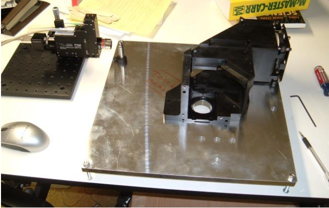
Fig. 11 The PSM focused on the center of a steel ball sitting on the post located in the bored hole in the aluminum alignment plate.

In the case of the spectrometer the same approach is used. First a post and ball are placed at the center of curvature of the collimating mirror. The PSM on a 3 axis stage is placed facing the mirror and adjusted until the objective focus is at the center of the ball in all 3 degrees of translational freedom. Half inch diameter, Grade 5 steel balls are excellent convex mirrors. The ball is removed from the post so the light from the objective illuminates the mirror and is refocused near the objective focus. The 3 screws on the mirror are used to bring the center of curvature of the mirror to the precise focus of the objective in all 3 degrees of freedom. This is why 3 adjustment screws are needed on the mirror so that the mirror can be adjusted not only in 2 angles but axial translation to get best focus as well.

This step is repeated for the decollimating mirror. The post is moved to that hole in the plate, the PSM is moved over and focused on the center of the ball, the ball is removed, and the mirror adjusted with the 3 screws. Note how the PSM is used to place an optical conjugate that cannot be touched physically in proper relationship to a feature that is mechanical and can be touch probed mechanically. The PSM is a transfer device from an ethereal optical conjugate to a rigid mechanical datum, or vice versa.

Now the fold mirrors can be adjusted by using holes located where the centers of curvature should appear as reflected in the correctly adjusted fold mirrors. In Fig. 11 there are a set of 4 holes toward the front edge of the alignment plate. The hole nearest the edge of the plate is where the center of curvature of the relay mirror is after the fold mirror is installed in the black optical bench. The idea is the same for the spectrometer. The PSM is set up facing the fold mirror and centered on the ball. The fold mirror is then adjusted in 3 degrees of freedom until the center of curvature is centered on the PSM focus. Notice that it takes 3 adjustments on the plane fold mirror to accomplish this alignment.

Once both fold mirrors are adjusted a post and ball can be placed where the exit slit is to go, and the PSM aligned to a ball at the entrance slit as in Fig. 12. Only if the grating is adjusted so the double pass reflection of the entrance slit lies on the exit slit will light return to the PSM focus. This 0 order reflection from the grating establishes the zero angle setting on the grating rotation axis and allows a correction for any tilt in the orthogonal direction.

Another aspect of this final alignment is that the return spot to the PSM will not be a perfect spot but will be aberrated due to the optical design of the spectrometer. But the aberrated spot should be of a size and shape consistent with the design of the spectrometer. If it is not the expected spot it is clear something is wrong with one or more of the optics. Actually, at each previous step in the alignment a serious figure error in any of the optics will be noticed. The PSM has the ability to sense asymmetry in the image down to a level of 1/8th to 1/10th wave. If there are figure errors of these magnitudes, they will be apparent in the “Star test” image10, 11,12 as each of the optics is aligned. This means that errors in assembly can be caught before the entire system is put together, and before having to figure out which element is to blame for the lack of system performance.
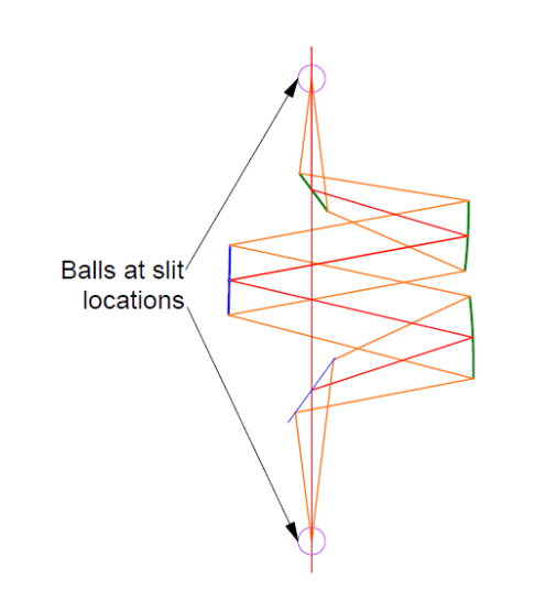
Fig. 12 Check of the grating zero angle by double passing the spectrometer off a ball at the exit slit

Conclusion

We have explained what an autostigmatic microscope is, and how it can be used for measuring optical surface radii. I have also described how a modern version of an ASM was developed over a number of years as my familiarity with its use expanded and as technological advances were made in many useful components that became part of the final Point Source Microscope. Finally we showed an application of using the PSM for alignment of optical components and showed how an ASM acts as a transfer device from ethereal optical conjugates to fixed mechanical references.

References

1 Steel, W. H., “The Autostigmatic Microscope”, Optics and Lasers in Engineering, 4, 217-27, (1983). 

2 Drysdale, C. V., “ON A SIMPLE DIRECT METHOD OF DETERMINING THE CURVATURES OF SMALL LENSES”, Transactions of the Optical Society of London, pp. 1-12, 1900.

3 Smith, W. J., Modern Optical Engineering, 3rd ed., McGraw-Hill, New York, (2000), p. 584.

4 Malacara, D., Optical Shop Testing, 3rd ed., Wiley & Sons, NJ, (2007).

5 Korsch, D., Reflective Optics, Academic Press, San Diego, CA, (1991), p. 15.

6 Gaertner Scientific, https://www.gaertnerscientific.com/microscopes/main.htm

https://directory.eoportal.org/web/eoportal/satellite-missions/s/skylab

8 Parks, R. E., “Optical tests using fibers, balls and Ronchi gratings”, OSA OF&T Workshop, Mills College, Oakland, CA (1980).

9 Smith, W. S., “Versatile interferometer for shop use,” Proc SPIE 192, 16 (1979).

10 Malacara, op. sit., pp. 398-420, particularly pp. 418-9.

11 Richard, H., Star testing astronomical telescopes, William-Bell, Inc. (1997) pp. 9-13.

12 Parks, R. E., “Using image symmetries to uniquely align aspheric mirrors to a focus and axis”, Proc. SPIE, 12222, 1222205 (2022).
Free Psm Data Logging Software Available

A user of a PSM mentioned that it was too bad that data of spot positions could not be logged in the PSM Align software. This is true, data cannot be logged in the PSM Align software, but there is a version of the software designed for use with the centering station, LCS-PSM Align, that does log data. We do not send this version of the software out with the PSM alone because we figure it is not needed, at least initially, and it just adds more to the time to get familiar with the PSM.

On the other hand…

If you have a need to log data versus time as in a drift test to monitor changes with temperature or other environmental factors, we will gladly send you to a link where you may download the LCS-PSM software. Another place where this software is useful is if you have an application where a device is moved at a constant velocity, you can log spot position data versus a time base on the assumption that equal time intervals are proportional to scan distances. The advantage is that there is no need for a software connection between the LCS-PSM software and the scanning software or actuation device. This means you can set up a scanning situation without getting a software engineer involved to connect two sets of software.

Anyone desiring a link to the LCS-PSM software should email info@optiper.com and we will send you a link to the Installer and instructions for installing the software. You do not lose any of the PSM functionality and can still use the PSM standalone software.

For a very short video showing the spot motion and logging see below:

Rapid Centering Of Optics

ABSTRACT

Traditionally a rotary table is used for optical centering because the table creates an axis as a reference. Previously, we showed that a Bessel beam also creates an axis useful for centering. The Bessel beam axis and a center of curvature of a surface makes it possible to center an optic simultaneously in tilt and decenter. We also showed that simultaneously sampling two arbitrary points along the Bessel beam also permits full adjustment of tilt and decenter of a powered optic. This makes centering possible without either a rotary table or a precision linear stage. In most common instances, however, sampling the beam at two points is unnecessary because of the inability to correct for both tilt and decenter. We discuss an alternative, simpler method using a Bessel beam.

1. INTRODUCTION

Traditionally a rotary table is used for optical centering. When a reflection from a center of curvature is stationary as the table rotates, the center of curvature lies on the rotary table axis. When both centers of curvature of a powered element are stationary as the table rotates, the element is free of both tilt and decenter. To measure this lack of motion requires a precision rotary table and a linear stage to move between the centers of curvature. The actual centering is slow and tedious because you must sample first one and then the other center of curvature, iteratively, to remove tilt at one conjugate and decenter at the other while keeping track of the azimuth of the rotary table so you move efficiently in the proper direction toward sufficiently small motion at both centers of curvature. The process is further complicated because the tilt correction affects the decenter and vice versa. In many cases you have to overshoot the apparent correction at one conjugate to move to centering the other. Needless to say the process begs for simplification.

Previously we showed that using a Bessel beam1 as reference axis would eliminate the need for a rotary table for centering2. This means simple x-y motions of the element being centered are guided by reflected spot movements on a video screen. This directly couples alignment motions of the element in a particular direction with visual feedback from a video screen showing complementary motions in the same azimuthal direction making for efficient and intuitive hand/eye coordination. By sensing the position of the Bessel beam and a reflection from the center of curvature of the element in the same plane, the optical axis of the element is defined by a point and two angles. Overlapping the two spots on the axis of previously aligned crosshairs guarantees the optical axis of the element lies on the Bessel beam reference axis.  Using this method, a powered optical element can be fully centered in tilt and decenter quickly and without iteration.

However, the method is not entirely free of error. If the initial element in an assembly is not perfectly aligned in tilt and decenter the Bessel beam transmitted through the element will no longer be perfectly aligned with the reference Bessel beam before the first element was installed. This will lead to small errors in the centering of subsequent elements. This is not to say that equivalent errors also occur using a rotary table, but for best practice the method should eliminate or minimize these errors. Another short coming of this method is that for elements with centers of curvature close to the element, the sensor must be close to the element and that interferes with access to the element for centering, cementing and cleaning. What would be ideal would be a method where the sensor was positioned relatively far from the element being centered.

In an attempt to overcome these deficiencies we first came up with a method that uses the benefits already described, but uses them in a way so that the sensor is a sizable distance from the elements being centered. Further, the sensor is fixed at that distance for the entire centering process of one or more elements. In this method3, an optical trombone is placed between the lens being centered and the sensor so the Bessel beam can be sampled at two axially separated points. By sampling the beam at two separated points the displacement as well as the angle of the beam are determined giving enough information to completely center a lens both in tilt and decenter.

The method worked well and just as expected, but as we used the method to center lenses we realized the approach was overkill in the sense that in most cases of centering there is no means of adjusting the lens in both tilt and decenter. This new method gave more information than was useful in practice.

The other feature of the method was that in sampling just one point along the Bessel beam the method was quite sensitive to errors in centration. Because the sensor could be placed relatively far from the lens being centered there was a substantial optical lever arm that made the method sensitive. Thus for practical reasons, and the idea that simpler is better, we decided not to use the optical trombone, but to use a single point of reference on the Bessel beam to determine best centering. 

In this paper we describe why a majority of lenses can only be centered in either tilt or decenter. Certainly there are very high quality lenses where there are sufficient adjustments to achieve centering in both degrees of freedom, but we limit our present discussion to the majority of lenses in consumer products where a lens can only be centered in one degree of freedom.

We show the theory of centering in one or the other degrees of freedom in terms of their sensitivity to centering errors in terms of first order optical lens parameters. Then we show the calculated sensitivities match those predicted by the theory.

2. PRACTICAL CONSTRAINTS TO CENTERING

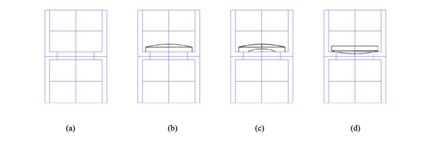
Most lens cells have a seat and a bore nominally centered on the axis of the cell as shown in Fig. 1a. Also, most assembly takes place using gravity to hold the lens down to the seat. This is why we do not consider the case where the seat is above the lens. In Fig. 1b we show a plano-convex lens sitting on the seat. This lens can always be perfectly centered to the cell by sliding the lens on the seat independent of how well the lens optical axis is concentric with its edge (up to the point that the periphery of the lens hits the side of the cell). 

rapid centering of optics fig1

Fig. 1 A typical lens cell with seat and bore (a), a plano-convex lens sitting on the plane seat (b), a meniscus lens with an edged flat sitting on a plane seat (c) and a spherical surface sitting on the bore in the seat (d)

On the other hand it is clearly impossible to tilt this lens provided the seat is perpendicular to the axis of the cell. In Fig. 1c we have much the same situation, but here the flat on the lens resting on the seat was added by edging and an error in tilt could be introduced during edging. As with case 1b, the lens can only be adjusted by translation but how well it can be centered depends on how well the flat on the lens is perpendicular to the axis of the lens. The difference in cases 1b and 1c, relative to centering, are that edging tolerances matter in the case of 1c but can be loose for 1b up to the point of mechanical interference with the cell.

In Fig. 1d, the lens, whether it is plano- or bi-convex, can be centered perfectly by tilting alone as long as the bore in the seat is perfectly centered to the cell. If the bore is centered and the seat perpendicular to the cell axis, the lens rotates about the center of curvature of the surface resting on the seat. That means the center of curvature necessarily lies on the axis of the cell. As the lens is rotated about the center of curvature of the surface on the seat, the center of curvature of the opposite face can always be brought onto the axis of the seat, again as long as the edge of the lens does not hit the cell wall.

A ray of light coming from under the lens and centered on the cell axis will not be deviated by the lower surface because it hits the surface at normal incidence. When the lens is rotated in the seat until the center of curvature of the upper surface also lies on the axis of the cell, the ray strikes the upper surface at normal incidence and is undeviated. Again, edging tolerances can be loose as long as there is clearance to center the lens by tilting about the bore in the seat. In this scheme the tight tolerances are placed on the cell and getting it well aligned to the centering fixture.

3. SENSITIVITIES TO ALIGNMENT

3.1 Plano surface on the seat

Assume that the cell is made perfectly and is aligned perfectly to a centering fixture such that the cell mechanical axis is coincident with a Bessel beam projected from under the lens. Light from infinity parallel to the cell axis would come to focus at the back focus of the lens in Fig. 1b. If the lens is centered on the Bessel beam the beam will also pass through the back focus4. If the lens is slid a distance, d, to the right, the back focus will move d to the right and the Bessel beam will deviate so that it also passes through the shifted back focus. This means the deviation of the Bessel beam is just 

α = d/efl,      (1  

where efl is the effective focal length of the lens. 

With a collimated beam of light this shift of the back focus can only be sensed in the plane of the back focus. With a Bessel beam, the position of the beam can be sensed at almost any distance from the lens except in the vicinity of the back focus because there the beam expands to an annulus. If the lens has an efl of 10 mm but the viewing microscope is 100 mm from the lens, a 1 μm decenter of the lens will be seen as a 10 μm motion of the spot in the microscope. The angular deviation of the Bessel beam behaves as d/efl for any power of lens, positive or negative, the only difference being which way the Bessel beam moves relative to the lens axis.

3.2 Spherical surface on the seat

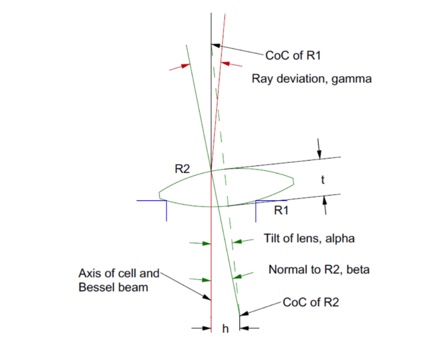
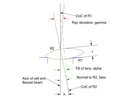
If a spherical surface sits on the seat as is the case in Fig. 1d the only means of centering the lens is to rotate it about the center of curvature of the surface on the seat. Calculating the deviation of the beam is a bit more complicated than in the case of decenter. Consider Fig. 2 with a bi-convex element tilted by an angle α. The center of curvature of R2 then lies a distance

h = (R1 – R2 – t)sin(α)      (2  

from the axis of the cell. This means the normal, β, to R2 is h/R2 and after refraction at R2 the deviation of the beam deviation is

γ = [(n – 1)(R1 – R2 – t)sin(α)]/R2      (3  

Equation (3) says the deviation is directly proportional to the lens tilt, α, and to a term related to the shape factor of the lens in the sense that as long as [(n – 1)(R1 – R2 + t)/R2] remains constant, the deviation is independent of the lens focal length.

rapid centering of optics fig2

Fig. 2 The ray deviation of a tilted lens with a convex surface on a centered seat

For example, as the surfaces become more concentric, the angular deviation goes to zero. For a plano convex lens as in Fig. 1d, the deviation is α/2 independent of the efl while for an equi-convex lens the deviation approximately α independent of the efl. Just as in the case of decenter, the deviation may be measured at almost any distance from the lens except in the vicinity of the back focus so that there is good sensitivity to the deviation of the Bessel beam.

There are practical limitations to how far the sensor can be from the lens. As the sensor is backed away from the lens the Bessel beam becomes less intense and the sensor views a larger area of scattered light so there is a decrease in signal to noise at large distances. However, the use of the Bessel beam makes possible a situation that is impossible with conventional imaging, the ability to view the propagation of a single ray at almost any axial distance. This is what makes the use of the Bessel beam so powerful and lets you move the sensor well above the cell so there is space near the cell to work and inspect the assembly.

4. EXPERIMENTAL VALIDATION OF CENTERING SENSITIVITIES

4.1 Case of decentration only

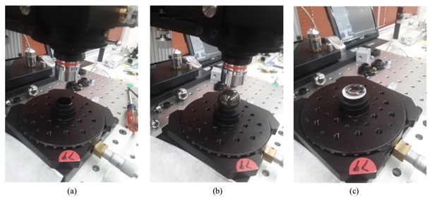
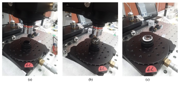
In order to test the simulation in Section 3 we used a catalog lens, nominally a 200 mm efl plano-convex lens. The seat for the lens, shown in Fig 3a, was on an x-y stage so we could center the seat to a Bessel beam projected from under the seat. In Fig. 3b we used a ball and a Point Source Microscope (PSM)5 focused at the center of the ball to center the seat to the Bessel beam. The first step to center the ball was to determine the height of the ball center with the ball on the seat and set the PSM to that height. Then the ball was removed and the PSM was translated perpendicularly to the Bessel beam coming up from under the seat so that the crosshairs in the PSM were centered on the Bessel beam. Then the ball was replaced and the x-y stage with the seat was moved to center the ball on the PSM crosshairs. 

Fig. 3c shows the lens sitting on the seat convex side up and the microscope focused substantially about the lens. The first set of tests were made with the plano side on the seat as in Fig. 3c so the angular deviation of the beam should be strictly proportional to the lens efl. 

rapid centering of optics fig3

Fig. 3 The lens seat (a), the lens seat being centered using a ball (b) and the plano side of the lens on the seat (c)

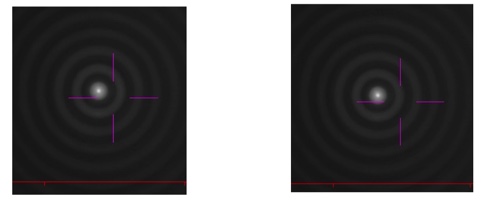
The first measurement was made with the PSM focused on the vertex of the convex surface with the lens closely centered with respect to the Bessel beam. The second measurement was made after decentering the lens by 1000 μm. The cropped images from the PSM video screen are shown in Fig. 4 where the tick marks on the red bar are 100 μm apart. Using the centroiding algorithm in the PSM it showed the spot moved about 8 μm right to left for a lens decenter of 1 mm in the x direction while a Zemax simulation of this case showed the spot should have moved 2 μm.

rapid centering of optics fig4

Fig. 4 Cropped images of the Bessel beam with the PSM focused at the vertex of the convex side of the lens. On the left is the beam position prior to decentering. On the right is the position after decentering 1 mm. The spot moved 8 μm

One might ask why did the spot move so little for a 1 mm decenter of the lens until you realize that when you are focused at the vertex of the lens you are only 0.4 mm above the 2nd principle plane, in this case, where there should be no motion of the spot. The second thing to realize is that if you can focus on the vertex and see the Bessel beam, you can also focus on the principle plane and see there is no motion in this plane. This means you can make a precision measurement of the efl rather than the bfl of any lens without the need for a nodal slide.

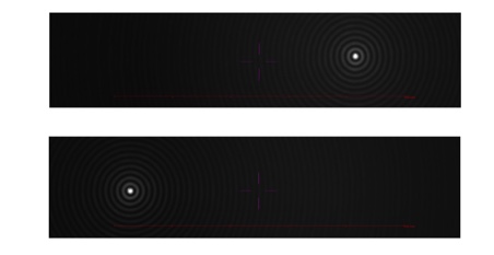
Next, the PSM was moved up to 100 mm above the vertex where the lens was again centered with respect to the Bessel beam and then decentered 1000 μm. This time the spot moved 488 μm and Zemax predicted a motion of 500 μm. Fig. 5 shows the spot motion. Because the motion was large we decentered the PSM to move the spot to the right initially so that the spot remained on the screen when it was decentered. Also, we had to leave the picture full size in the direction of the decenter for a comparison between the two situations. The PSM centroiding algorithm was used to measure the spot location before and after decentering.

rapid centering of optics fig5

Fig. 5 Bessel beam spot locations 100 mm above the lens centered (upper) and decentered by 1 mm (lower) showing a movement of 488 μm. Red tick marks 100 μm apart

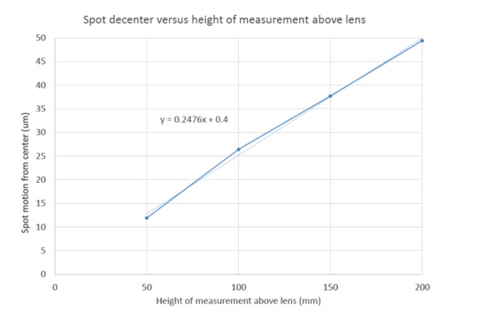
Moving up to 200 mm above the vertex, the decenter was reduced to 500 μm so the spots would not go off the screen. In this case the spots moved 491 μm while Zemax predicted 499 μm. If the spot motion is plotted against distance from the lens the slope of this line in 0.00487 where Zemax predicts a Bessel beam deviation of 0.00498. Above 200 mm the Bessel beam spot disappears because you are in the region of the back focus.  Once you get above this region for this longer focal length lens the Bessel beam spot lacks intensity to make a good measurement. On the other hand if a 500 μm decenter shifts the beam approximately 500 μm and you can measure the beam to a 1 μm sensitivity you have a sensitivity to decenter of about 1 μm. In angular terms this as about 1 second of arc, that is, 0.001/200 mm = 5 μradians ~ 1 second.

To recap, for decenter, the angular beam deviation is just the decenter over the efl and the spot motion is the deviation times the distance above the lens the measurements is made. If the measurement distance is close to but less than the bfl, the Bessel spot displacement is very close in magnitude to the amount of the decenter.

4.2 Case of lens tilt only

The other case is tilt of the lens when the powered side of the lens sits on the seat. With the equipment at hand it was difficult to directly measure the tilt of the lens in the seat. The experiment was modified so that we decentered the lens and modeled what that decenter did to the angular beam deviation using Zemax. For a 50 μm decenter of our 200 mm efl lens, Zemax predicted the beam deviation was 0.02354°, 1.41 arc minutes or 411 μradians. For the constant 50 μm decenter the spot position was measured every 50 mm above the lens.

rapid centering of optics fig6

Fig 6 Bessel beam shift as a function of distance above the 200 mm efl lens

Again the measurement can be taken at any convenient height above the lens as long as it is not close to a back focus. Since the decenter we used was equivalent to a lens tilt of 411 μradians and the spot moves about 50 μm when measured 200 mm above the lens we have a measurement sensitivity of about 8 μradians to tilt for this lens assuming a 1 μm sensitivity to spot displacement, far better than needed for all but the most precision lenses. In addition, if we look back at the equation for the beam deviation for this lens we find the deviation γ = 0.585α and our α = 411 μradians so γ is 240 μradians, almost the same as the slope of the graph in Fig. 6 taking into account the slope is shown in units of μm/mm.

5. CONCLUSION

Once we realize that for most centering there is a single degree of freedom, either tilt or decenter, the whole problem of centering is vastly simplified if we also take advantage of the property of Bessel beams to propagate as though they were a single paraxial ray. Then the beam deviation or decentration can be measured at almost any practical distance above a lens or lens assembly without ever having to move the measurement device. Further, whether the centering error is tilt or decenter, either can be measured on the order of 1 μm or 1 second of arc if you have the ability to measure the Bessel beam position to 1 μm. This ceases to be true for very short focal length lenses but one can always use a higher power objective to give greater sensitivity to spot motion.

It has already been noted that centering without the need for a rotary table was 5-6 times as fast as using the rotary table6. The drawback to the method proposed there was that the vertical column on the centering device either had to be very good, or very well calibrated. By using a Bessel beam that propagates like a single paraxial ray there is no need for the precise column. The sensing unit is put at a convenient height and never moved throughout the centering process. As always in the case of optics, one size never fits all, but almost all cases can be covered with this method.

REFERENCES

[1] Durnin, J., “Exact solutions for nondiffracting beams. I. The scalar theory”, JOSA-A, 4, 651-4 (1987).

[2] Parks, R., “Alignment using plane Axicon gratings”, Proc. SPIE, 10747, 1074703 (2018)

[3] Parks, R., “Practical considerations for using grating produced Bessel beams for alignment purposes”, Proc. SPIE, 11816, 1181603 (2021)

[4] Parks, R., “Design for alignment”, Proc. SPIE, 11103, 1110302 (2019)

[5] https://optiper.com/en/products/item/point-source-microscope

[6] Heinisch, J., Hahne,. and Langehanenberg, P., “Rotation-free Centration Measurement for Fast and Flexible Inspection of Optical Lens Systems”, Proc. SPIE, 11175, 111751B (2019)

Practical Considerations For Using Grating Produced Bessel Beams For Alignment Purposes

ABSTRACT

Bessel beams are useful for alignment because they create a small diameter, bright, straight line image in space perpendicular to the Axicon, or Axicon grating, producing the beam that is an exact analog of a single ray in a ray tracing program. Here we limit our discussion to Bessel beams produced by plane gratings whose pattern is evenly spaced concentric circles that are illuminated by a point source of light on the grating axis. The gratings produce a more nearly ideal Bessel beam than a lens type Axicon, and the plane grating serves as a plane mirror as well in an alignment setup so the combination define four degrees of freedom in space rather than the usual two.

Most discussions of Bessel beams assume illumination with collimated light. We have found it advantageous to use a point source for illumination because it is easy and less expensive to use a single mode fiber as a source than a precision collimating lens the diameter of the Axicon. Besides, collimated illumination produces a Bessel beam of finite length in transmission while in theory a beam of infinite length is created using a point source.

With these assumptions about how the beams are produced and details about the grating diameter and line spacing it is easy to calculate the useful length of the Bessel beam in reflection from the grating, the usual matter of concern when using the grating for alignment purposes in a double pass test setup. Other practical matters are also discussed such as lens centering with a test apparatus with no moving parts.

1. INTRODUCTION

Credit for the discovery of Bessel beams generally goes to back to Durnin1 in 1987, but really the credit should go to McLeod2 in 1954 where he describes the invention of the Axicon because the beam created by an Axicon is a Bessel beam. Unfortunately for McLeod he did not have a laser at his disposal and so the bright spot created by his Axicon did not show much (any) of the structure surrounding the bright spot and he did not realize he had stumbled on this new form of light beam. Besides, McLeod was a very practical person primarily interested in alignment of optical systems, not the physics of the beam produced by the Axicon3.

Even after McLeod wrote a second paper4 describing uses of the Axicon for alignment there was not much interest in Axicons until Durnin’s1 sparked an interest because of the so-called non-diffracting nature of Bessel beams. Also, Durnin and his coworkers were initially creating their Bessel beams not with Axicons, but rather with opaque screens with a narrow annulus that created the Bessel beam on the axis of the annulus. This led Vasara5 to realize Bessel beams could be created by plane gratings, in part, to make the beam more efficient in terms of light through put by using the full aperture instead of just an annulus.

In spite of several papers6,7,8 including the widely distributed Optics & Photonic News9 mentioning uses of Bessel beams for alignment, virtually all the interest in Bessel beams has been in other areas of optics, astronomy and physics. There seems to be almost no interest in this simple yet powerful technique for the practical, everyday alignment uses such as cementing doublets and centering optics in a barrel, let alone aligning optics in 2 and 3 dimensional space where alignment becomes more of a challenge particularly if it has to be done precisely. The purpose of this paper is to attempt to illustrate some of the practical concerns of using Bessel beams so it is easier for others to take advantage of this powerful alignment technique.

2. WHAT IS A BESSEL BEAM AND HOW IS IT PRODUCED?

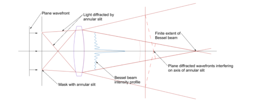
Before getting into the practical issues of using Bessel beams it makes sense to review what Bessel beams are and how to produce them. Referring to Fig. 1, a plane wavefront is incident on a narrow annular aperture centered on and at the back focus of a lens.

practical considerations fig1

Fig. 1 Creating a Bessel beam using a plane wavefront and an annular slit at the back focus of a lens (after14)

This is how Durnin, et. al. 1 created their Bessel beams. In the plane of the page, the lens collimates the light from the upper portion of the slit to produce a plane wavefront progressing downward from the lens that has a width of the slit diameter, while the lower portion produces a plane wavefront of the same width progressing upward. Since the picture is symmetric about the axis of the annulus and lens, these two wavefronts produce a set of nested cones of light in the region where the wavefront overlap. 

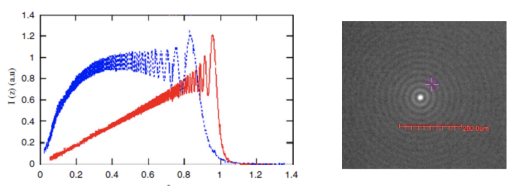
The phase of the light at the apexes of the nested cones interferes constructively along the axis creating a line of light whose intensity is much greater than in the region surrounding the axis. This bright line is the core of the Bessel beam and is the useful portion for centering. The intensity of the light in the core along the axis varies in an oscillatory manner and gets less intense near the lens but never goes to zero as shown in Fig. 2a. Perpendicular to the axis the light also varies in rings of diminishing intensity away from the bright core as shown in Fig. 2b.

practical considerations fig2

Fig. 2a Variation in intensity of the Bessel core in the direction of propagation for a plane wavefront (red) and converging wavefront (blue) (left ) from reference 11 and Fig. 2b variation in intensity perpendicular to the axis of the beam (right)

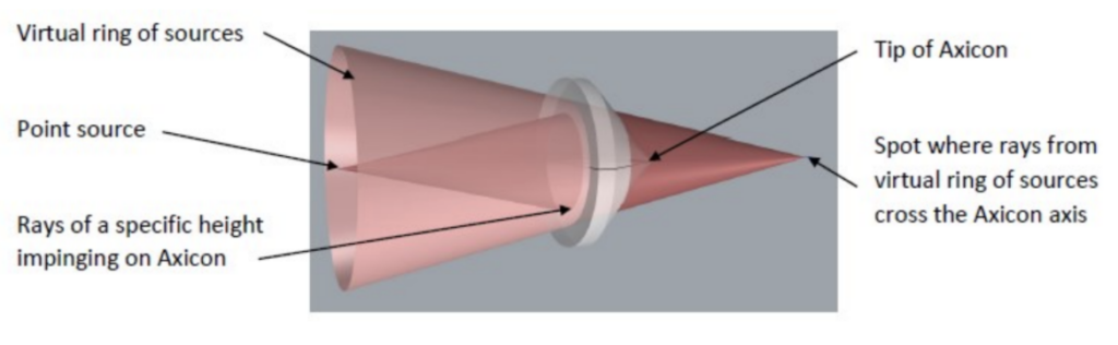
From a practical standpoint, the Durnin method of using an annulus is inefficient because most of the aperture of the lens is obscured. A physical, cone shaped glass Axicon as McLeod used also creates a Bessel that uses all the light incident on the clear aperture of the Axicon. Fig. 3 illustrates how the Axicon creates a nested set of cones of light although only one is shown because making a figure with many cones is difficult. For each different ray height of the spherical wavefront impinging on the Axicon a different diameter ring of virtual sources is created that cross the axis of the Axicon at a different distance from the tip.

practical considerations fig3

Fig. 3 Illustration of how a conical Axicon creates the nested cones of light to form a Bessel beam

A third way of creating a Bessel beam is to use a pattern of equally spaced, concentric rings printed on a photomask substrate, in other words, a computer generated hologram (CGH)5. This can be pictured similarly to Durnin’s approach but no lens is needed. Looking at the pattern of circles edge on with the center of the pattern in the plane of the page, the pattern acts like a linear diffraction grating to an incident plane wave. A small amount of light goes straight through the grating as the 0 order while much of the rest of the light is diffracted into + and – first orders at an angle of λ/d where λ  is the wavelength of the incident light and d is the pattern line spacing. Now the nested cones are made up of the + 1st order light as the page is rotated 360 degrees around the axis of the pattern.

Roughly 40% of the incident light goes into the transmitted Bessel beam for a binary grating pattern and 40% into the reflected beam. While this is less efficient light wise than a physical Axicon, the CGH has 2 distinct advantages over the glass Axicon. First, the CGH is also a plane mirror and therefore simultaneously defines 5 degrees of freedom, 3 translations and 2 angles, a great advantage to anyone doing alignment. The second advantage over the cone shaped Axicon is that the grating pattern is almost perfect in the sense that CGHs can be written with an rms precision on the order of 1 part per million or better10 over a scale of spatial wavelengths of at least 10^4. 

There are two questions that may be asked about the precision, what about wavelength of illumination and the flatness of the substrate. First, the Axicon gratings work at any wavelength. You can create a Bessel beam with white light. Regarding substrate flatness, it is hard to imagine a low order deformation that will affect the straightness of the Bessel beam. Power and astigmatism may affect the shape of the rings around the core but it would have to be an error like the “S” shape of coma before the straightness of the beam would be affected, and this high an order of deformation is difficult to induce mechanically.

A final comment of the relative advantages of a conical glass Axicon versus a grating. At the present time a physical Axicon 25 mm diameter is less expensive than a similar size grating in unit quantities by perhaps a factor of 2. In some cases they are essentially the same price. Because the grating Axicons can be produced by contact printing the price will become much less expensive with higher volumes. Since Axicon gratings are “perfect” and more flexible to use than true conical Axicons the balance of the discussion will be limited to grating Axicons.

3. DESIGN AND USE OF AXICON GRATINGS

When Axicons are discussed the immediate mental picture is that they are illuminated with a collimated light source. Most of the literature assumes this because it is a little easier to describe the theory. However, use with a collimated source limits the scope of use and the ease of implementation. First, a good lens the same diameter as the Axicon is needed to collimate the incident light. Second, the collimated input limits the theoretical length of the transmitted Bessel beam. Using a point source of light a known finite distance from the grating permits a Bessel beam in transmission of almost any length. Because any Axicon makes relatively inefficient use of the light incident on it, a laser source is almost a necessity in practice to produce a long Bessel beam. 

An adjustable 1 to 10 mW laser diode source coupled into a single mode fiber makes an ideal source with which to illuminate the grating via a free space coupling. Such a fiber patch cord in the visible will have a near perfect Gaussian output with a NA of about 0.1. This source placed about 125 mm behind a 25 mm diameter grating gives about optimum coupling to the grating, at least for illumination purposes. This convenient set of initial parameters will be used now to examine the Bessel beams produced by these constraints. It will be obvious how to deviate from these values depending on the specific situation.

A next obvious question is the line spacing of the pattern. I made a reasoned guess at 10 μm lines and spaces to give a grating spacing of 20 μm. Using this spacing with 635 nm light gives λ/d = 0.03175 = 1.815° = α. It has turned out that this was a good choice. Gratings with this spacing are easy to make and the diffraction angle seems to be useful for all applications I have tried so far. This is not to say there will not be a case where another spacing is a better choice but I cannot see anything wrong with this choice, at least as a good place to start.

3.1 Properties of the Bessel beam in reflection

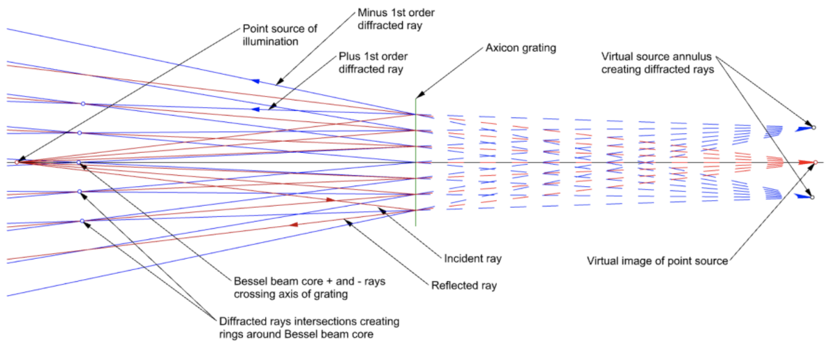
Because the grating line pair spacing of 20 μm has worked out well it will be used for further discussion. Also, it has been convenient to size the grating at a 25 mm diameter so we’ll use that as well in the example but a practical upper limit would be 140 mm for a 6 x 6” photomask substrate. If we put a point source of light a distance z = 125 mm in front of an Axicon grating with 20 μm/lp spacing and illuminate it with 635 nm light we have the situation in Fig. 4 where we assume the grating radius is 12.5 mm = Rmax, and the diffraction angle was increased to 5° for clarity. 

practical considerations fig4

Fig. 4 Creation of a Bessel beam by a point source in reflection from an Axicon grating

Light rays (red) from a point source at the left of Fig. 4 reflect from the Axicon grating. The reflected rays appear to emanate from a virtual point source at the right of the figure. On either side of the reflected rays are plus and minus 1st order diffracted rays (blue) that appear to emanate from a virtual annulus in the plane of the virtual point source. The radius of the annulus is the distance z from point source to grating times the tangent of the diffraction angle α. Diffracted rays from equal and opposite sides of the axis of the grating interfere on the axis of the grating to form the core of the Bessel beam while rays from opposite sides of the axis but different heights at the grating interfere to create the rings around the core.

By looking at the rays impinging on the center of the grating it is clear that there will be ray crossings starting immediately to the left of the grating to form the beginning of a Bessel beam in reflection. As the ray heights increase on the grating the diffracted ray crossings proceed to the left until they reach a height of 4 mm, for our example, where the crossing extends to infinity. Beyond that the diffracted rays start to diverge and create virtual crossings to the right of the grating that mimic the real crossings to the left of the grating.

For the reflected Bessel beam the usual method of creating and observing it would be to use an autostigmatic microscope (ASM) with the point source in the microscope illuminates the Axicon grating and observes the reflected Bessel beam. In this case the reflected Bessel beam length never exceeds the distance from the focus of the ASM to the grating and this distance will be limited by the diameter of the grating. The maximum distance the ASM can be from the grating is limited by the zonal radius of the grating. Once z = Rmax*tan(α) = 393.38 mm, for our example, the virtual annulus is at infinity with a radius of Rmax. As z increases from there the virtual annulus moves to the left of the grating and the diffracted rays diverge so they never enter the ASM objective. The other 1st order rays are always diverging. This means when using an ASM with an Axicon grating in reflection the maximum length of the Bessel beam will be Rmax*tan(α). Since Bessel beams are self-healing12 a point inside the limit just stated will create a Bessel beam to the left of the source provided the source does not obscure too much of the beam.

Another practical aspect of moving the ASM too far from the grating is the objective will have a reasonable NA, typically about 0.3 for a 10x objective. As you move farther from the grating the intensity of the illumination is decreasing as z^2 which is not bad in and of itself, but as the source illumination is increased scattered and ambient sources of light increase the background illumination around the core. The point here is to use the reflected Bessel beam to align the ASM to the grating and then align a point source on the other side of the grating to the ASM to create a longer length useful Bessel beam13. Because the point source creating the transmitted Bessel bean can be placed close to the grating the illumination is intense and the beam as mentioned earlier can go to infinity in theory. 

3.2 Properties of Bessel beams created in transmission

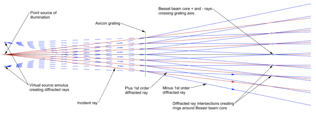
Fig. 5 shows what happens when a point source illuminates the grating in transmission. Assume the source is still at 125 mm from the grating but the diffraction angle is 5° to spread the rays for clarity. The Figure shows a point source illuminating the grating with the 0 order rays (red) passing through the grating. On either side of each transmitted ray are plus and minus 1st order diffracted rays (blue) that appear to emanate from an annulus of radius z*tan(α) surrounding the point source. As with the reflected ray case, the diffracted rays on either side of the grating axis and the same height at the grating cross the axis to create the core of the Bessel beam. Rays from differing heights at the grating form the rings around the core.

practical considerations fig5

Fig. 5 Bessel beam formation in transmission using a point source of illumination

 As long as the point source is closer to the grating than Rmax/tan(α) the Bessel beam propagates from the grating to infinity. This means the Bessel beam created in transmission can be used with greater flexibility than the reflected beam but there does not appear to be a good method of assuring the axis of the Bessel beam is strictly perpendicular to the grating other than aligning the transmitted beam to an ASM that has been previously aligned using the reflection mode. If not aligned in this manner the Bessel beam can be several degrees off perpendicular without affecting the quality of the beam14. In some applications the alignment with the grating makes no difference, for example, when using the beam to determine straightness. However, if the beam is used for alignment it is usually necessary for the beam to be perpendicular to the grating.

3.3 Other practical considerations concerning using Bessel beams

3.3.1 Axicon grating light efficiency
Axicon gratings are not very efficient light wise. At any particular observation point along the Bessel beam you are only seeing the light that make it through an annulus the width of the annulus. For example, the ring at 4 mm radius where the diffracted rays are normal to the grating has an area of 0.2516 mm2 and rings inside this are progressively smaller. This is why the intensity shown in Fig. 2a is low close to the grating. For this reason a SM fiber coupled light source with a variable intensity of several mW is a practical size source. The source does not have to be monochromatic, or even close to monochromatic, to create a Bessel beam. White light will work if you can get enough into a fiber to get useful light in the diffracted beam.

3.3.2 Use of Bessel beams with quad-cells
Keeping with the ring size topic, using a Bessel beam with a quad-cell does not work. The energy spread around the central core is close to uniform because every ring has nearly the same energy as the rings on either side of any particular ring15. The reason it is easy to center on the central core with a digital camera is that the energy density is about 8x greater than in the first ring. When the camera shutter speed is set to give a threshold of about half the peak intensity of the core, the only pixels above the threshold are pixels in the core and centroiding is a simple as finding the center of gravity of the pixels above threshold.

3.3.3 Ease of initial alignment with Bessel beams
On a related topic, because there is energy spread out laterally way beyond the core it is easy to know which way to adjust a mirror or lens to bring the core into the field of view of the microscope objective used to view the Bessel beam. As the intensity of the light source or the shutter speed is decreased, the rings around the central are visible even though the central core is many mm outside the typical field of view of about 1 mm for a 10x objective and modest size format digital camera.

The best way to think about this advantage is to think about aligning an autocollimator to a plane mirror a couple meters away. It is a 2 person job in a darkened room using a flashlight shining in the eyepiece. Once reflected light is back in the objective the job is done, but getting the light in the aperture of the autocollimator is a real trick. With the Bessel beam the rings are a flag waving to tell you which way to tilt the mirror to get light in the aperture even though you are grossly misaligned to begin with.

3.3.4 Aligning point source to the grating axis
The point source illuminating the grating must be on the axis of the grating within limits that are, in practice, fairly loose otherwise the core of the Bessel beam brakes up into a checkerboard pattern of dots. The details of how far off axis are given in this paper by Bin and Zhu16. A method of perfectly aligning the point sources to the grating in either reflection or transmission was previously given13.

In addition, the central core also breaks up if the Bessel beam goes through or is reflected from an optic that introduces sufficient aberration. For example, if a lens is sufficiently tilted relative to the Bessel beam the astigmatism introduced will break the core into a pattern of dots. There is still information in the pattern but it is much harder to interpret than the central core. Again, this topic is beyond the scope but some insight may be gained from Bin and Zhu16. In practice it takes a wavelength or 2 of aberration before there is an effect on the core.

3.3.5 Commercial availability of Axicon gratings
Finally, for those who want to experiment with Axicon gratings they are available commercially for reasonable prices17. If the use of these gratings grows the price is bound to come down.

4. METHOD OF USING A BESSEL BEAM TO FIND TILT AND DECENTER SIMULTANEOUSLY

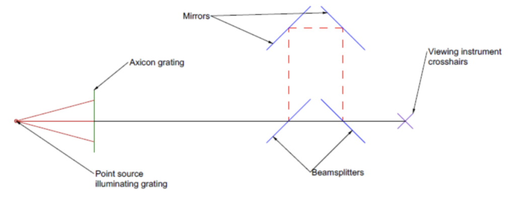
As a final topic on practical uses of Axicon gratings we describe a method for determining the centering and tilt of a lens without moving anything but the lens itself in 4 degrees of freedom. The principle behind the method is that if we know the location of two points in space we know the origin and slope of the line between the points. What is needed is a device that will sample a Bessel beam simultaneously at two points along the beam. One way of sampling the Bessel beam at two axially displaced locations is to use an optical trombone where one light path goes straight through (blue) while the other (dashed red) is diverted through the trombone to increase its optical path length as shown in Fig. 6. The light arriving in the focal plane of the observing instrument, usually a microscope, comes from two axial locations along the Bessel beam separated by twice the distance of the fold mirrors to the beamsplitters. Before inserting the trombone beam sampling device, the viewing microscope crosshairs are centered on the Bessel beam coming from the Axicon grating. Then the sampler is inserted in the beam. The sampler, depending on the type of beamsplitters used, will shift the beam more or less from the crosshairs if it is not well aligned in angle. Once the sampler is aligned the beam passes through the sampler undeviated as in Fig. 6.

practical considerations fig6

Fig. 6 Axial beam sampler aligned with a Bessel beam and microscope

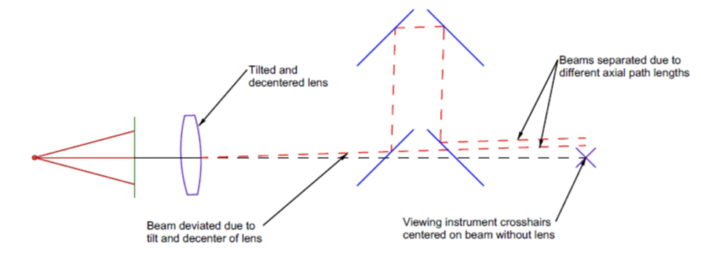
Adding a tilted and decentered lens element between the grating and the sampler will displace the beam at the microscope focal plane but by different amounts depending on whether the beam has travelled the long or short path as shown in Fig. 7.

practical considerations fig7

Fig. 7 A tilted and decentered lens inserted between the Axicon grating and the axial beam sampler producing different displacements of the two beams at the focal plane observing microscope

In order to align the lens in both tilt and decentered to the viewing instrument, both central cores of the Bessel beams must lie on the microscope crosshairs. If the observing instrument has a resolution of <1 μm (typical of a Point Source Microscope18 with a 10x objective) and the distance between axial observing locations is 100 mm the lens can be centered to <1 μm and aligned parallel to the axis of the beam to <2 seconds of arc without having to move any part of the observing instrument. The advantages of aligning lenses without having any part of the alignment apparatus move other than the adjustments to the lens itself are obvious for improving productivity.

5. CONCLUSION

We have explained how Bessel beams are created using Axicon gratings and have shown how to calculate the useful range of the beam in reflection. There is no practical limit to the range in transmission. In addition, we have discussed several practical considerations for the use of Bessel beams for alignment in conjunction with observing instruments that use digital cameras. In particular, the ease of alignment if the setup is initially badly misaligned so no bright light is in the sensor field of view. It was pointed out that Axicon gratings are commercially available and that the quality of the Bessel beam produced is a higher quality than those produced by conical axicons although the gratings are only about half as efficient in light use.

Finally we showed how to precision align a lens element in tilt and decenter by using an optical trombone to sample the Bessel beam at two axially separated locations. The technique improves productivity because there are no moving parts in the alignment setup and adjustments to tilt and decenter can be dialed in with adjustment screws.

REFERENCES

[1] Durnin, J., “Exact solutions for nondiffracting beams. I. The scalar theory”, JOSA-A, 4, 651-4 (1987).

[2] McLeod, J. H., “The Axicon: A New Type of Optical Element”, JOSA, 44, 592-7 (1954).

[3] (Personal opinion from meeting McLeod in 1967 at Eastman Kodak Company.)

[4] McLeod, J. H., “Axicons and Their Uses”, JOSA, 50, 166-9, (1960).

[5] Turunen, J., Vasara, A. and Friberg, A., “Holographic generation of diffraction-free beams”, Appl. Opts., 27, 3959 (1988).

[6] Vasara, A., Turunen, J. and Friberg, A., “Realization of general nondiffracting beams with computer generated holograms”, JOSA A, 6, 1748 (1989).

[7] Fortin, M., Piche, M. and Borra, E., “Optics test with Bessel beam interferometry”, Opts. Express, 12 5887 (2004).

[8] Gale, D. “Generacion y aplicacion de haces Bessel en trabajos de alineacion”, Rev. Cub. Fisica, 27, 28 (2010).

[9] Jaroszewicz, Z., Burnall, A. and Friburg, A., “Axicon-the Most Important Optical Element”, Optics and Photonics News, April 2005, p. 34.

[10] J. Ye, M. Takac, C.N. Berglund, G. Owen, R.F. Pease, “An exact algorithm for self-calibration of two-dimensional metrology stages”, Prec. Eng., 20, 16, (1997).

[11] Dong, M and Pu, J., “On-axis irradiance distribution of axicons illuminated by a spherical wave”, Optics & Laser Tech., 39, 1258 (2007).

[12] Bouchal, Z., Wagner, J. and Chlup, M., “Self-reconstruction of a distorted nondiffracting beam”, Optics Communications, 151, 207 (1998).

[13] Parks, R., “Alignment using axicon plane gratings”, Proc. SPIE, 10747, 1074703, (2018).

[14] McGloin, D. and Dholakia, K., ‘Bessel Beams: Diffraction in a new light”, Contemporary Physics, 46, 15-28, (2005).

[15] Durnin, J., Miceli, J. and Eberly, J., “Comparison of Bessel and Gaussian beams”, Opt. Lett. 13, 79 (1998).

[16] Bin, J. and Zhu, L., “Diffraction property of an axicon in oblique illumination,” Appl. Opt. 37, 2563-2568 (1998).

[17] https://optiper.com/en/products/buy/axicon-grating

[18] https://optiper.com/en/products/point-source-microscope

Need Custom Optical Test Equipment?

WHY START FROM SCRATCH WHEN YOU CAN ORDER A PSM FROM OUR WEBSITE?

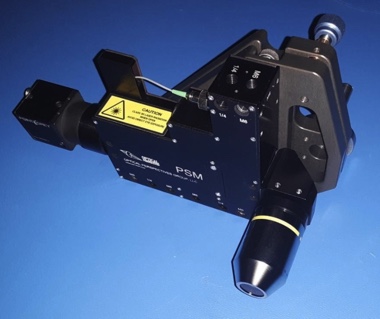
It may surprise you but about 15% of Point Source Microscopes (PSMs) purchased are built into custom optical test hardware. Optical Perspectives supplies a CAD model of the PSM to help the customer integrate the PSM into their test hardware design. When the custom hardware is built the PSM is bolted in place, connected to its computer and the test hardware is ready to use as an autocollimator, alignment device or centering sensor.

COTS APPROACH 

This COTS approach reduces the time and cost of custom optical test hardware by avoiding the development and procurement phase of obtaining a precision sensor and software for optical test equipment.

The PSM is compact and lightweight so it is easy to mount to almost any structure via the many tapped mounting holes in its body. Two USB connections to a computer with installed and proven PSM Align software is all that is needed to be up and running.

If a change is needed in the software to optimize the PSM for your application it is easily made on industry standard, LabVIEW™ based, PSM Align software. Optical Perspectives will even provide the source code if a customer wants to introduce their own modifications.

PSM FORM FACTOR 

The PSM coupled with its custom, precision tip/tilt mount and right angle adapter is an autocollimator with better than 1 arc second resolution.

In this configuration, the output beam can be oriented 360 degrees relative to the PSM body and the total package has a form factor of 160 x 110 x 54 mm and a mass of about 1 kg.

For use as an alignment or centering sensor the PSM has a form factor of 200 x 110 x 32 mm and a mass of less than 1 kg. 

PSM form factor lg

PSM CONFIGURED FOR MOUNTING ON A CMM IN PLACE OF THE TOUCH PROBE

There are also adapters to mount the PSM in other centering devices or for mounting as the sensor on a CMM in place of a touch probe.

Use with a CMM is ideal for aligning complex, precision optical systems to assure that all components are positioned exactly to design to CMM accuracies.