New Product Launch
Optical Perspectives Group proudly introduces PSM Align
Revolutionary Python-Based Software for Point Source Microscope
Now Standard on All PSM Units

Author: csadmin

Chapter 9: Creating and Viewing Single Paraxial Ray

From the beginning we have said that centering a lens meant aligning the optical axis of the lens to a reference axis. Up to this point we have assumed the axis was the mechanical axis of a rotary table. Because there are disadvantages to using a rotary table, I was curious to see if there was another way to create a reference axis. The path to a new axis came from the subject we have been discussing, the cementing of doublet lenses. The idea also came from my interest in computer generated holograms (CGH) for use as calibration artifacts for coordinate measuring machines and CNC machine tools. [1]

As we have discussed, the seat of the convex side of the meniscus half of a doublet determines the location of the center of curvature of that side. The center of curvature of the concave side is the second point defining the lens axis. It is easy to design a CGH of Fresnel zone patterns to serve as datums for cementing 3 balls to the CGH centered on a Fresnel zone of the correct radius to match the location of the center of curvature of the concave side looking through the lens. [2] A combination of the seat and center of curvature make precision centering the meniscus easy when a centering sensor is centered on the center of curvature.

A second Fresnel zone of a different radius is designed to focus at the same height when the positive element is placed on the meniscus. This means that the meniscus is first aligned and fixed in place and then the positive element aligned to the meniscus without ever having to move the alignment sensor. If the sensor does not have to move it cannot introduce errors due to its movement. Top and side views of such a CGH and doublet alignment scheme are shown in Fig. 1.
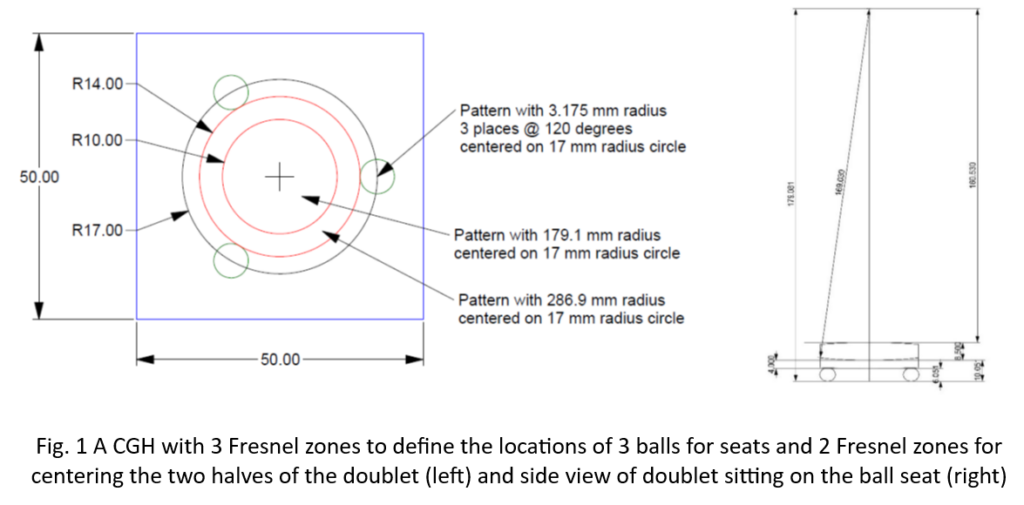
doublet alignment scheme

As you can read about the successful experiment in the reference there is no need for the details here. While the CGH did exactly what was intended it meant that a different CGH would be required for every different doublet design. Also, this design using balls to serve as a seat made it difficult to secure the aligned meniscus so it would not move when adding and aligning the positive element.

This success coupled with the use of a zone plate CGH to measure the straightness of travel of mechanical ways on machine tools [1] lead to the idea of using the “beam” of light created by the zone plate as a universal method of centering doublets and other alignment tasks. The concept of using a zone plate for alignment purposes is not new. In the 1950’s the Dutch optical scientist A. C. S. van Heel discussed the problem of aligning multiple points to a line because it is difficult to see all the points at once [3]. He goes on to suggest using diffraction by a slit for alignment in one axis before generalizing the idea to use a zone plate of evenly spaced concentric circles. He says that under good observing conditions alignment to 1 µradian is possible. [4]

In 1954, John McLeod of Eastman Kodak, also interested in alignment, invented the Axicon [5] in part to improve the light efficiency of alignment instruments. He said that by illuminating the axicon with a pinhole source of light it “will project a continuous straight line of image out to infinity.” In Fig. 1 of his paper, he shows a diagram that is very close to that in the paper by Durnin [6] that shows how an illuminated annular mask creates a beam of light coined by him as a Bessel beam.

Technology has made great progress since the days of van Heel and McLeod. The zone plates van Heel used were made by light grinding of rings in a polished glass plate to create rings that would transmit and block the light. The rings were typically 1 mm in width. Later the rings may have been made photographically but I could not find a reference. McLeod’s axicons were not the easiest optics to make either, and it wasn’t long after Durnin’s paper that Turunen, et. al. [7] showed that it was easy by then to make zone plates as computer generated holograms (CGH) with narrow line spacings.

It turns out in hindsight that both van Heel and McLeod were producing and using Bessel beams for alignment purposes. It took about 30 years for theorists to review their experimental results and add a theoretical explanation to the phenomenon described by the earlier empirical observations.

This is a good place to describe a simple Bessel beam as it turns out there are many variations. The simplest beam has an intensity distribution perpendicular to the direction of propagation proportional to the square of the 0 order Bessel function as in Fig. 2 (right), and the intensity distribution captured on a digital camera in Fig. 2 (left). The first ring of the pattern has 16% the intensity of the central peak, and the peak and each ring has the same radiant energy. This means it is easy to precisely centroid on the peak with a digital camera to a small fractional of a pixel if the peak covers a diameter of 3–4 pixels. Because the irradiance of the pattern is nearly constant, a quadcell is useless for centroiding.
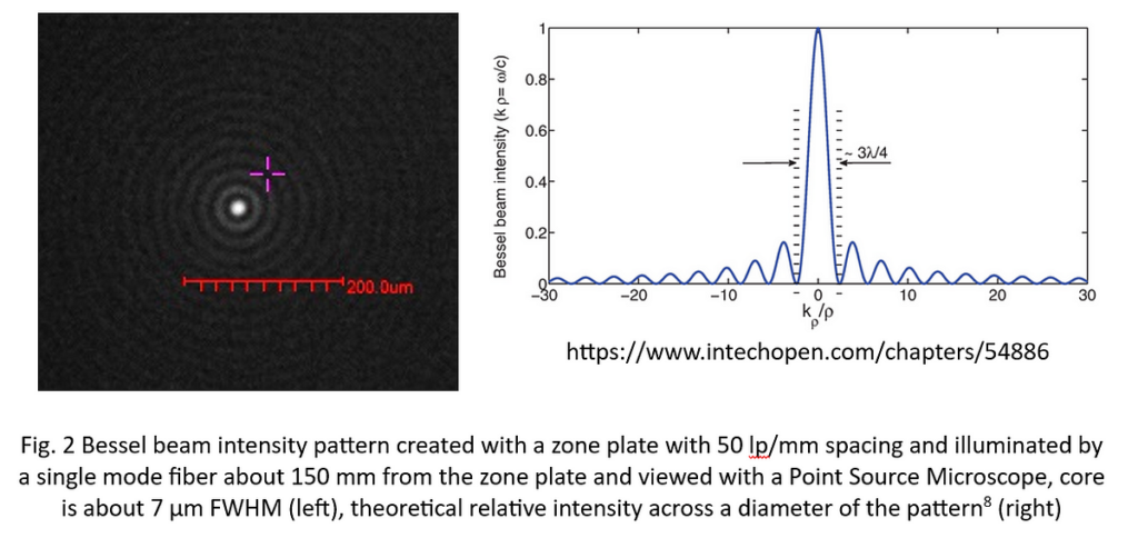
Most discussions of Bessel beams assume the illumination of the axicon, or zone plate is collimated. With collimated illumination the beam is a finite length. A point source of light is also a suitable source and produces a beam of close to infinite extent. The source does not have to be coherent or monochromatic. White light works fine. Each of these changes gives a slightly different formal name to the kind of Bessel beam and the ones I use by illuminating a grating with the end of a single mode fiber and laser diode source should probably be called Bessel-Gauss beams.

Now that I have described what a simple Bessel beam is and how they are produced we should get back to the way they propagate through optical systems and why they are useful for alignment. After some initial experiments over 3 years ago using the Bessel beams to measure the straightness of ways on machine tools and realizing errors in transverse motion of a fraction of a µm were easily observed, I began watching what happened when I moved a lens through the beam. I found that when my ASM was focused inside a lens at what appeared to be the principle plane, the transmitted beam did not move as the lens was moved perpendicular to the beam. It did move one way above the plane and the other on the opposite side of the apparent principle plane. This is paraxial rather than real ray behavior.

In the meantime, I found the paper “Propagation of generalized Bessel-Gauss beams through ABCD optical systems” [9] that implies the behavior I was seeing was paraxial. This prompted me to do an experiment with a ball lens and create the Bessel beam with a 50 lp/mm axicon grating from AOM. [10] A ball was used since it is always free of tilt and all I had to control was the decenter, or ray height, of the Bessel beam incident on the 8 mm diameter, BK7 ball.

In the experiment, [11] the ball lens and microscope were stationary, and the Bessel beam was translated across the ball close to the ball center to keep the experiment paraxial. For this BK7 ball with an index of 1.515 the efl is 5.8834 mm. If the ball is decentered 1 µm the ray will exit the ball at an angle of h/efl = .001/5.8834 = .00017 radians. The intersection of the entering and exiting rays was at the mid-plane of the ball, its principle plane. The experiment confirmed the paraxial behavior of the Bessel beam.
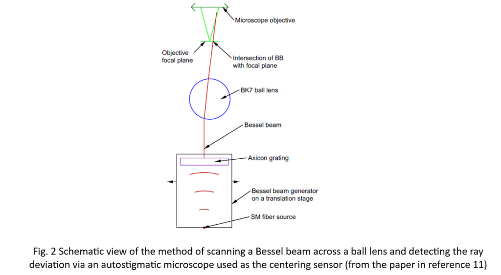
This paraxial behavior has profound consequences relative to alignment and to measuring lens properties in general. The transverse position of the beam can be measured anywhere along the beam including inside the ball, lens or system of lenses. Or far from the lens so a small angular deviation causes a large transverse displacement. Just like the classical textbook picture, Fig. 3, from geometrical optics, if the incident ray is parallel to the lens optical axis it changes direction at the second principle plane to cross the optical axis at the focal point of the lens. (The region right around the focal point is the only place the Bessel beam cannot be viewed because it turns into an annulus.)
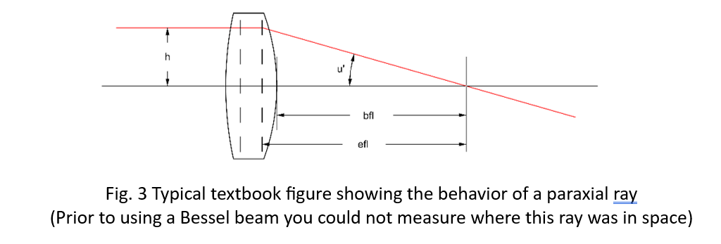
Because the Bessel beam behaves as a single paraxial ray it is easy to calculate the ray deflection angle due to decenter as simply the decenter over the efl. This immediately gives an idea whether a particular height above the lens will be sufficient to give the required sensitivity. If the lens sits in a centered seat, then tilt of the lens changes the ray angle by (R1/efl) times the lens tilt.

For our example meniscus a decenter of 10 µm changes the ray angle by .01/-110.66 = -9.04 µradians and a lens tilt of 1 mradian changes the ray angle by (264.97*.001)/-110.66 = 2.394 mradian. Not surprisingly lens elements with short focal lengths are more sensitive to misalignment than ones with longer focal lengths, or less power.

We have covered many topics in this Chapter, so it is time for a quick review.

· The expense and tediousness of using a rotary table for lens centering led me to look for an alternative method

· An initial use of a Fresnel zone CGH was successful centering but not practical

· Experience with zone plates made with CGH techniques for mechanical alignment led me to try them for optical alignment

· The Bessel beams made by the zone plates appeared to propagate through optical elements and systems as though they were paraxial rays

· Published works and further experiments convinced me the propagation was paraxial

· This meant the Bessel beam position could be measured anywhere along the beam

· In turn this means it is easy to measure the beam angle exiting a lens to find centering errors independent of where center of curvature are located

In the next Chapter we will look at more consequences of the paraxial behavior of Bessel beams and their application to centering and alignment.

References

[1] Parks, R., Ziegert, J. and Groover, J., Computer Generated Holograms as 3-Dimensional Calibration Artifacts, Proc. ASPE, 117–20 (2017)

[2] Parks, R. Optical alignment using a CGH and an autostigmatic microscope, Proc. SPIE, 10377, 1037708 (2017) also https://www.opticalperspectives.com/category/published-papers/page/3/

[3] van Heel, A. C. S., High Precision Measurements with Simple Equipment, JOSA 40 (12) 809 (1950)

[4] van Heel, A. C. S., ed., Advanced Optical Techniques, Wiley & Sons, NY, pp. 451–2 (1967)

[5] McLeod, J., The Axicon: A New Type of Optical Element, JOSA, 44 (8) pp. 592–7 (1954)

[6] Durnin, J., Exact solutions for nondiffracting beams. I. The scalar theory, JOSA A 4, (4) 651–4 (1987)

[7] Turunen, J., Vasara, A. and Friberg, A., Holographic generation of diffraction-free beams, Appl. Optics, 27 (19) 3959–62 (1988).

[8] Costanzo, S., https://www.intechopen.com/chapters/54886

[9] Santarsiero, M., Propagation of generalized Bessel-Gauss beams through ABCD optical systems, Optics Communications, 132 (1996) pp. 1–7

[10] Arizona Optical Metrology https://cghnulls.com/

[11] Parks, R. and Kim, D., Physical ray tracing with Bessel beams, Proc. ASPE Spring Topical Meeting 2023 (This paper is available as a sidebar to the Chapters on alignment at https://medium.com/@reparks_11319/introduction-to-a-series-of-articles-on-optical-alignment-4d2bf0282e33 )
Chapter 8: Alignment of 3 Centers of Curvature

A convenient and concrete example of aligning three centers of curvature is the cementing of the doublet we used in the optical axis example in Chapter 5, the details of which are reproduced below.

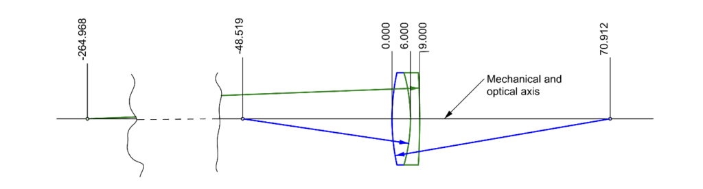
Fig. 1 Doublet used as an example of aligning three centers of curvature

The goal is to get all three centers of curvature on the same line to some tolerance dictated by the desired lens system performance. When alignment and centering is done in practice the meniscus element is placed on a seat with the concave surface facing up so that when a drop of cement is added it is contained within the concave well. We have already been over the details of aligning the optical axis, or two centers of curvature, of the meniscus to a seat in Chapter 7.

As seen in Fig. 1, the task now is to align the upper convex surface of the positive element so that its center of curvature lies on the optical axis of the meniscus. The interface between the two lens elements takes care of itself as the cement acts as a lubricant between the interface surfaces. The cement is worked out to a thin uniform thickness by pressing down and gently sliding the positive element around on the meniscus. Once the cement is thin enough that there is a drag resisting the sliding the positive element is centered and the cement cured.

Because the surface facing the alignment sensor and its objective is convex, the objective must have a working distance of more than the radius of the upper surface, or roughly 71 mm in this case. Unless the diameter of the lens being cemented is quite small, the convex surface will be longer than most commercially available microscope objectives. Autocollimator type centering sensors come with a variety of working distance objectives and autostigmatic microscopes can be fitted with simple doublet objectives to get the required working distance.

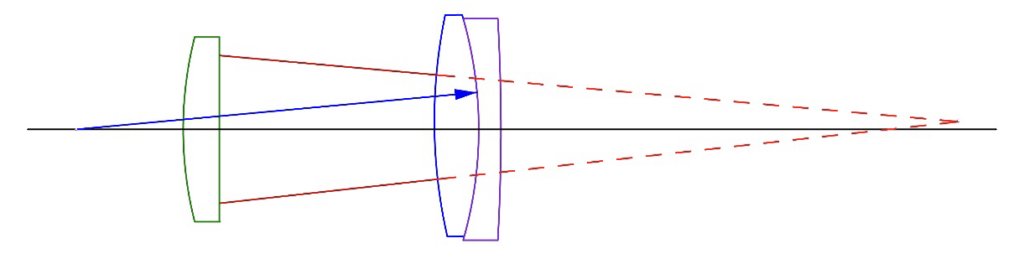
While using an objective with a long enough efl will almost always reach the center of curvature, there is a loss in sensitivity to alignment due to the increase in the focal length of the objective. For cementing doublets this is probably not an issue because the longer the radius, the weaker the lens and the less sensitive the lens is to alignment. There are cases where the doublet has a large diameter and is relatively fast where alignment can be an issue so there is a need for greater sensitivity. There are other occasions where there is physical interference, and a long working distance is needed to reach the center of curvature. In these cases, it is possible to add a 1 to 1 relay in front of the objective that has sufficient sensitivity. An example of such a relay for use with an autostigmatic microscope is shown in Fig. 2. This makes an aesthetically ungainly instrument but achieves the purpose of no loss of sensitivity.

Fig. 2 Long working distance objective with same lateral sensitivity as the microscope objective

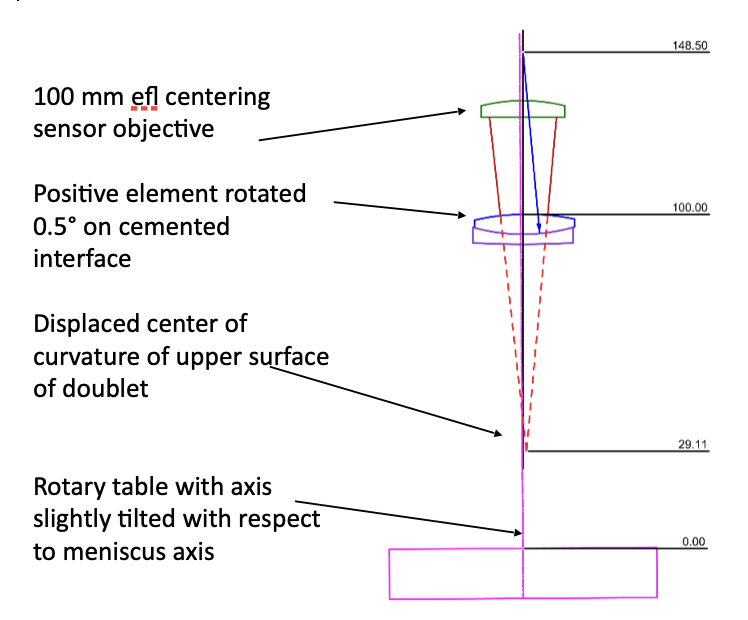
Going back to our example, assuming we use an objective with a 100 mm efl to reach the center of curvature of the upper surface, we have a situation as in Fig. 3. The 0.5° (0.0087 radian) tilt of the positive element moves its center of curvature 1.042 mm off the axis of the meniscus. Since almost any optical sensor can detect a µm decenter and there is a 2x magnification of the displacement due to reflection, the center of curvature location is easily measurable to 1 second of arc, better than any but the most stringent centering requirement.

Fig. 3 Light from a 100 mm efl objective reflecting from the 0.5° tilted positive doublet element showing the displaced center of curvature of the convex surface rotated about the interface surface

Figure 3 shows the mechanical implications of being able to center to 1 second of arc. From similar triangles, the positive element is about 1/3 of the distance from the objective to the center of curvature which implies that the edge of a perfectly centered element will be aligned to a perfect meniscus to about 1/3 of a µm, far better than such an element is realistically edged. 

What I am trying to illustrate here is that aside from very small (cell phone camera and endoscope lenses) and very large lenses, relying on mechanical tolerances of the edges of elements may not be the optimum approach where precision centering is needed. Optical centers of curvature are the critical features for alignment, not mechanical interfaces at the edges. The peripheral mechanical interfaces should be designed to allow for the adjustment of the centers of curvature, but these interfaces should not be the features that define the alignment when high precision is needed.

As an example, some doublets are centered and cemented using a “V” block to align the edges of the elements. Assume we want to align our example doublet to 3 minutes of arc or about 1 milliradian, a typical centering tolerance for good but not precision centering. This means that the 2 elements must be edged within 50 µm of the same diameter to meet this tolerance assuming no other errors in the centering process. If there is any wedge in either of the elements there will be additional errors. 

I think the idea of the use of optical versus mechanical features for alignment goes beyond the optical elements themselves. Consider the typical rotary table centering device. It uses a mechanical axis of rotation to define the reference axis to which we want to align our optical elements. In one sense this is an ideal method of centering as we have previously illustrated; if the transmitted or reflected image from an optical surface moves it does not lie on the axis of the rotary table, full stop. However, we have optical centering sensors that detect motion of an image to a fraction of a µm. That means the runout of the table must be less than a µm to make use of the full sensitivity of the sensor. 

In addition, the tilt or wobble, of the table must be small and the further the optic being centered is above the table the worse the effect may be. Assume our table has a 1 second of arc (5 µradian) tilt and the optic we are aligning is 100 mm above the table. As the table rotates the mechanical vertex of the element will translate ± 0.5 µm and if our sensor could see a mark at the vertex, it would be seen to move 1 µm TIR (total indicator reading, a terminology from mechanical touch indicators). 

However, our optical sensor is not viewing the vertex of the element but rather the center of curvature. In the case of our example doublet we have the situation in Fig. 4 where the center of curvature of the upper surface lies near the rotary table surface.

chap8 fig 4

Fig. 4 Misaligned doublet on rotary table having a tilt error

Since the center of curvature lies near the table and we assume that the tilt in the table occurs near the table surface, the motion of the center of curvature is reduced by the ratio of 29/100. The reverse is true of the interface surface, its CoC moves more by the ratio 148.5/100 and the CoC of the lower surface of the meniscus by 356/100. 

To minimize the errors in rotary tables they almost always are equipped with adjustment screws to remove the tilt and decenter that rotate in synchronism with the table. Errors of a higher frequency than once per revolution cannot be removed by these adjustments, however. The precision of alignment using a rotary bearing as the reference axis is never better than the quality of the bearing.

If the quality of the rotary bearing limits the precision of centering, what if the lens remained stationary? Then the quality of the vertical slide becomes the limiting factor because you must rely on its precision to move the sensing unit from one center of curvature to the other to establish the axis of the lens. This is not a new idea and was proposed in a paper1 a few years ago. The paper points out the advantage of this method. Assuming a sufficiently high precision vertical stage, the method is much faster than using a rotary table because there is immediate feedback of the result of making a centering adjustment.

When a rotary table is used you make an adjustment and then rotate the table to see if the adjustment has improved the centering. If the lens is stationary, you are making the adjustment to drive the reflected image to a particular position in the sensor coordinate system and can directly see how fast and far the reflected spot is moving without worrying about rotating the table. The paper estimates that eliminating the rotary table would speed up the alignment process by a factor of 5-6. To the best of my knowledge a product has never been brought to market based on this method. This may indicate that the method is not easy to implement in this form despite its apparent advantages.

The idea has merit, however. It depends on how the vertical slide is designed and implemented. Think of the possibility of using the vertical ram (the arm of the machine the probe is attached to) of a coordinate measuring machine (CMM) as the vertical slide. Even relatively inexpensive CMMs read out the probe location to ± 1 µm. This does not mean the probe moves with µm straightness, but that the calibration method and software tell you where the probe is in 3 degrees of freedom (DOF) to on the order of ± 1 µm plus a factor for the distance moved. Compared to the price of a precision centering device with a rotary table, a CMM with an optical sensor may be a cost effective method when it is balanced with productivity improvement. You only purchase the hardware once; you pay for labor every day.

Using a CMM for centering2 still means you must raise and lower the ram to go from one CoC to the other. The adjustment at each CoC is much faster than with the rotary table it but will still take more than one look at each CoC to make sure the best alignment is achieved. Further, the method still depends on precision mechanical motion and calibration. What if centering to remove tilt and decenter could be done without having to move any part of the centering measuring device? What if the only adjustments were the 4 that adjust tilt in 2 DOF and decenter in 2 DOF. The method would be faster and more precise. 

I have hinted at the method in Chapter 5 where we define the optical axis of a multi-element system as a line in space representing a single transmitted ray that is unchanged in location or direction when the lens is inserted in the ray path. In the next Chapter I will talk about how to generate a single ray that is useful for aligning optical systems in general but specially for centering of lenses to an optical reference axis.

1 J. Heinisch, F. Hahne, P. Langehanenberg, “Rotation-free centration measurement for fast and flexible inspection of optical lens systems,” Proc. SPIE 11175, 111751B (2019)

2 https://www.youtube.com/watch?v=FoeMAT8PfjU

Chapter 7: Centering 2 Centers of Curvature

In the previous chapter we looked at finding a single center of curvature using any of several optical instruments. This locates a particular point in space but does not define an axis. For that, two centers of curvature separated by a finite axial distance must be located to define an axis, or line. This chapter is devoted to finding an axis based on locating two centers of curvature simultaneously.

We resume with the assumptions from the previous Chapter that we have a rotary bearing table with its axis vertical and our optical sensor centered on the axis of the table looking downward at the table as was shown in Fig. 1 of Chapter 6. The sensor must be mounted on a vertical slide moving parallel with the table axis to reach the two centers of curvature. 

(Sidebar – Presumably an alignment telescope could be used to view the centers of curvature by adjusting the focus knob rather than moving the instrument along a vertical stage. Because of the mass, size and lack of video cameras I have never seen a rotary table centering instrument built using an alignment telescope. There may be such a configuration but I am unaware of it.)

This situation presents us with our first alignment task, the vertical slide needs adjustments in angle and position so the viewing instrument it carries moves parallel the axis of the rotary table as it is raised and lowered. To do this alignment optically we need an optical element sitting on the rotary table that has two separated but accessible centers of curvature along its optical axis. The BK7 element 10 mm thick shown in Fig. 1 is an example of an element that will work to produce the two centers of curvature. 

Obviously, there will be a reflection 100 mm from the concave side. Looking into the concave side, the 175 mm convex surface looks like its center of curvature is about 249 mm above the concave surface giving 2 spots 149 mm apart, good enough to discern the angle of the vertical slide to about 1 second of arc when we measure the centers of curvature lateral position to +/- 1 µm precision.pastedGraphic.png

Fig. 1 An optical element with 2 easily accessible conjugates to use to find the axis of a rotary table

You do not need a lens design program to do the calculation for a single element. If the left hand surface is R1 then its apparent center of curvature looking into R2 is R1optical = -R2(R1-t)/((R1-t)(n-1)-nR2) = 248.52 mm where n for BK7 at 640 nm is about 1.517. For more complex systems, a 1st design spreadsheet is very useful, and we will talk about some tricks to use with 1st order design in a later Chapter.

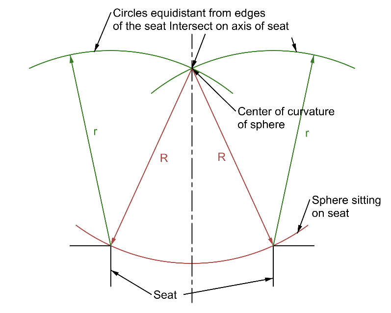
The two centers of curvature are easily viewed with either an autostigmatic microscope, or an autocollimator with an auxiliary objective of a suitable working distance. The element in Fig. 1 that you want to center is sitting in a seat that has adjustments for centering the seat relative to the table axis. With R1 sitting on the seat, the center of curvature of R1 will lie on the axis of the seat because a circle of any radius less than the radius of the sphere will lie on the surface of the sphere with the normals to the center of the circle passing thorough the center of curvature of the sphere as I have tried to indicate in Fig. 2. Thus, tapping the edge of the element in Fig. 1, or red circle in Fig. 2, will tilt the lens about the  center of curvature of R1 and the center will never move off the axis of the seat. The idea in Fig. 2 is obvious but just because it is obvious is often overlooked. The concept is very important to centering.

Fig. 2 Center of curvature of sphere on seat lies on the axis of the seat

Of course, tilting the lens element in Fig. 1 by tapping will move the center of curvature of R2. To center R2 you must decenter the seat. The procedure to center the lens and seat is the same basic procedure as aligning an alignment telescope to an axis as discussed at the end of Chapter 3. In this case, the axis of the rotary table is our reference axis. We look at the apparent center of curvature of R1 since it is farthest from the point of rotation of the lens in the seat and tilt the lens by tapping on its edge until the reflected image is stationary as the table rotates. The image does not have to be centered on the crosshair in the viewing instrument, it just must be stationary as the table rotates to assure the image is on the axis of the table.

Then you move the viewing instrument on the vertical slide to the center of curvature of R2 and decenter the seat until the reflected image is stationary. Again, the image need not be centered, just stationary. This adjustment will invariably throw the center of curvature of R1 off the table axis. These steps are repeated iteratively by tilting the lens when focused at the center of R1 and decentering the seat when focused at the center of R2 to bring the two centers of curvature onto the table axis. The centering is finished when each of the two centers of curvature remain stationary as the table rotates.

Each adjustment will bring the centers closer until the centering meets some specification for the tilt and decenter of the lens where the element in Fig. 1 is an analogue of a lens. A skilled operator centering much the same lens element will quickly learn that you generally want to undershoot, or depanding on the lens shape, overshoot, the adjustment to bring the lens to complete centration more quickly. You must also keep track of the azimuth of the rotary table so you don’t undo the previous adjustment by tapping on the wrong side of the lens. Centration to bring the optical axis of the lens coincident with the axis of the rotary table is tedious but is as precise as the bearing of the rotary table and the patience of the operator. This is why this method of centering using a rotary table has been used for over a century. In a subsequent Chapter we will talk about an easier way to do centering without the need of a rotary table.

A decided short cut in the method is to know the seat is well centered to the rotary table axis in the first place as is obvious from Fig. 2. Then the only adjustment to the lens is tilting by tapping on the edge while looking at the optical center of curvature of R1. Effectively, having the seat centered orthogonalizes the centering process in that the decentering is completed and only tilting is necessary to finish the job. This idea is the reverse of the bond ring method mentioned in Chapter 6. There the lens was cemented in the bond ring free of tilt so only decenter was left to correct.

It is still wise to check that the center of R2 is still centered before assuming the job is done until you have enough experience to be sure there is no need to check. The least burr or contamination on the seat will ruin the assumption that the seat is acting as if it were centered. 

To recap the points of centering an optical axis of a lens element to a rotary table axis we need:

  • A fixed focus optical sensor capable of projecting a crosshair or point source of light and detecting the return image of the projected source
  • The sensor must be mounted on a vertical stage and centered above the axis of a rotary table
  • The two centers of curvature of the lens element must be accessible to the sensor by moving the sensor along the vertical stage and/or by changing the objective lens of the sensor
  • There must be means of adjusting the lens in both decenter and tilt
  • When the reflected images of both centers of curvature are stationary (within some acceptable tolerance) in the sensor as the table is rotated, the optical axis of the element is coaxial with the axis of the rotary table
  • If the lens in incapable of being both tilted and decentered, or only one center of curvature is accessible, it is impossible to fully center the lens unless the seat accepting a spherical surface of the lens is well centered to the axis of the rotary table and the center of curvature that is opposite the one sitting on the seat

Before finishing this Chapter I should say that we have been discussing centering a lens optically on a rotary table. Mechanical centering is possible and is often used particularly for larger diameter lenses. Reviewing this method will reinforce what has been said about optical alignment.

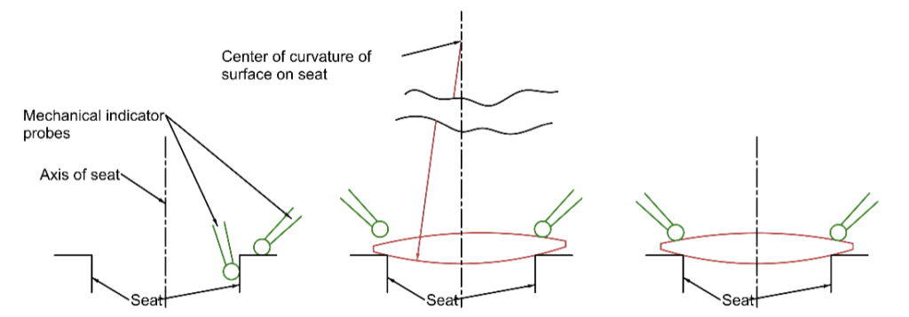
To center a lens on a rotary table the seat is first centered on the table using mechanical indicators to assure the seat runs true to the table as in Fig. 3. 

Fig. 3 Mechanical center of a lens on a rotary table

On the left of Fig. 3 mechanical indicators are used to assure the seat is running concentric and perpendicular to the axis of the rotary table. When the lens is first set on the seat it is clearly tilted and decentered, so the indicator shows a tilt or wedge in the lens as the table rotates. However, the center of curvature of the surface on the seat lies on the axis of the rotary table. As the lens is centered it rotates about the center of curvature until the indicator on the edge of the lens shows no height variation as the table and lens rotate. Then the center of curvature of the upper lens surface also lies on the axis of the table. Note the tip of the indicator remains the same height from the seat as the table rotates.

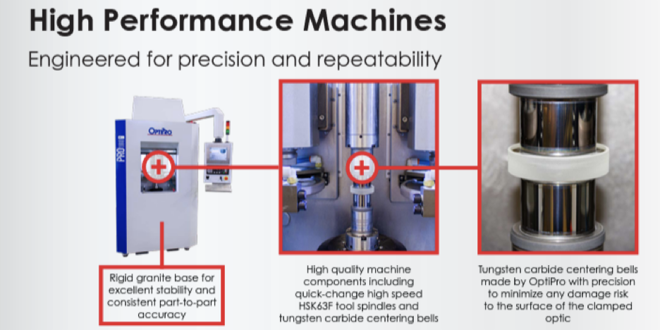
This also illustrates how bell cup centering machines work where lenses are made, see Fig. 4. The surfaces of the lens are squeezed between well centered cups to force the axis of the lens onto the axis of the cups. Obviously, this technique works best for steep bi-convex lenses and least well for meniscus lenses. The good news is that centering is most critical for lenses with considerable power and less so for weak lenses. The same holds true for centering in general but these are cases where the centering between pairs of weak lenses is critical because the wavefronts between the lenses have substantial spherical aberration.

Fig. 4 A screen shot from OptiPro’s website of bell centering cups seen squeezing a lens in the right hand photo

(I am not trying to play favorites here. Many optical machine manufacturers make similar machines. This company just had a picture that perfectly illustrates the point I was making.)

Chapter 6: Centering on a Single Center of Curvature

In this Chapter we will discuss the centering of a single center of curvature of a lens in a cell sitting on a rotary table that creates a reference axis. This discussion describes the traditional method of centering a lens in a cell. While this does not sound like an ambitious goal, the ideas presented here set the context for all the alignment topics to follow. We will get into much more complicated situations later, but it makes sense to walk before we run so that we understand the principals involved.

A rotary table was used for centering long before anyone heard of optics. Rotary tables, lathes or bearings are used to make objects that have no variation in the normal distance from the axis of the table as the table is rotated. If there is a method of measuring the height variation, we say the object is round and centered when no variation in height is observed normal to the axis of rotation by a fixed indicator or measuring device. 

Notice there are two assumptions, one implicit; the object must be round, no azimuthal height variation and implicitly, the bearing true. The proper combination of a non-round object and poor bearing behavior can make it look like the object is centered. We will assume we have a perfect bearing so that any motion observed that is synchronous with the table rotation indicates decentration. This also implies that our centering will never be better than the bearing precision in tilt and decenter.

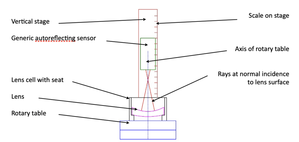
Using a rotary table introduces a practical constraint. In most cases the axis of the table is vertical so that gravity works for us. There are many examples where this is not the case, but for centering during the assembly of optics it is almost universally the case. The optical instrument, or sensor, viewing the optics being centered is mounted on a vertical slide centered on the axis of the rotary table. A scale to measure the height of the sensor that has a resolution consistent with the precision of the spacing of the lenses in the cell completes the hardware as shown schematically in Fig. 1

chapter six img 01

 Fig. 1 Schematic diagram of a rotary table lens centering apparatus 

The viewing, or sensing, instrument projects a point source of light, or an illuminated reticle, toward the lens being centered. When the projected source is at the center of curvature the light is normally incident on the upper concave surface and reflects back to the focal plane of the sensor and into an eyepiece or onto a monitor screen for viewing. As the rotary table revolves the reflected image will precess synchronously with the table unless the center of curvature is precisely aligned to the rotational axis of the table. The reflected image may not lie on the axis of the sensing instrument, but this only means the sensor in not well aligned to the axis of the table. If the image is stationary, it is on the axis of the rotary table. Fig. 2 helps with this explanation.

chapter six img 02

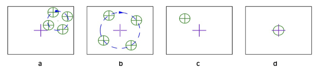
Fig. 2 Four possible alignment situations as the rotary table rotates the lens in Fig. 1

(The purple cross is the origin of coordinates within the sensor field of view, the black outline)

In Fig. 2a the center of curvature of the lens is not on the axis of rotation of the table nor is the sensor centered with respect to the table. In Fig. 2b the center of curvature is not centered on the table axis but the table axis is aligned with the coordinate origin of the sensor. In Fig. 2c the lens center of curvature is centered on the table axis because there is no motion as the table rotates but the axis of the table is not centered with the sensor origin, while in Fig. 2d the lens is centered and the table axis is centered with the sensor. In either case 2c or 2d the lens is centered with respect to the rotary table axis and that is all that is necessary for this one conjugate to be perfectly centered. That the reflected image does not lie on the center of the sensor has no effect on the centration of this surface of the lens. 

When the reflected image precesses with the table, then the center of curvature does not lie on the axis of the rotary table as in Fig. 3a. There are 2 ways to move the center of curvature onto the table axis. Referring to Fig. 3b, we can decenter the cell and lens pair until the image is still. Alternatively, we can rotate the lens about the center of curvature of the surface sitting on the seat as in Fig 3c and decenter the cell to keep the lens from interfering with the cell. Either method, or a combination of the two will center the image, but this does not mean the optical axis of the lens (magenta dotted line) is concentric with the axis of the table, only that the center of curvature of the upper surface is coincident with the axis of the table at a single point. Only when the cell is centered, and the lens rotated about the center of curvature of the surface against the seat are the 2 axes coincident. There must be sufficient clearance between cell and lens to make up for centration errors during edging the lens or the lens hits the cell, 2d.

Fig. 3 With center of curvature not on the table axis (a), and on the axis (b, c and d) 

Since we are only looking at one reflection for the moment, is there a way of completely centering the lens in Fig. 1 in the sense that it is free of tilt and decenter relative to the rotary table axis? Fig. 2d suggests that if we break the alignment into two parts, the answer is yes. First, we get the seat centered to the table axis using either mechanical or optical means. The centered seat and cell are locked to the table and the lens inserted. Since the seat is centered on the axis of the table, the surface of the lens sitting on the seat must also be centered. 

To finish centering the lens we must tap the edge of the lens to tilt it in the seat until the reflection from the center of curvature of the upper concave surface remains stationary as the table rotates. The axis of the lower surface remains on the axis due to the mechanical interface between the lens surface and the seat while the upper surface is free of tilt via the optical reflection.

As a bit of a sidebar, this technique that separates the operations of removing decenter separate from tilt orthogonalizes the centering. A derivative of this method is called mounting lenses in poker chips or bond rings. These mounts are accurately parallel with seats parallel to the outer surfaces. Jump ahead to Fig. 4a to see what a bond ring with a convex lens might look like. Notice that the convex surface center of curvature will always lie on the axis of the bond ring. Tilting about the center of curvature of that surface will bring the center of curvature on the axis of the bond ring if there is clearance.

Assuming the surface of the rotary table is precisely normal to the axis of rotation and the seat of the bond ring centered, the lens can then be inserted and made tilt free as above by using a reflection from the center of curvature of one or the other surfaces. The optical axis of the cemented bond ring/lens pair is then precisely normal to the parallel faces of the bond ring. If all the lenses in an assembly are prepared in the same way, then the whole assembly is aligned by simply removing decenter as each addition element is added to the assembly. This method is often used to assembly the lens elements in large lithographic systems, and a close analog is used to assemble microscope objectives.

Whenever precise centration is needed in a lens system the bond ring approach should be considered. It gives the necessary adjustment needed to correct for both tilt and decenter while not having the procedure of adjusting for one upset the other. The adjustments are separate and orthogonal. The method does involve extra metal parts, but these additions are generally more than offset by ease and precision of assembly. Also, a design may only have one critical interface as far as alignment goes. Use the bond ring idea only where it is necessary,

To finish up this discussion, look again at Fig. 3. When adding the second lens to the assembly we must assume the seat is not completely concentric to the rotary axis. This means that when we attempt to center the lens, we only have the option to tilt the lens to center it. There is nothing we can do about the decenter. This leaves the question of what is the best tilt for optimum performance of the lens system. Currently in our discussion there is nothing to do but tilt the lens until the center of curvature is stationary. In a later chapter we will show there may be a better option for best centering.

There are analogous situations where the only option is to decenter the lens as in Fig. 4b when the interface is a flat on the lens, the usual situation when the curve is concave. Here it is impossible to tilt the lens if the flat is not perpendicular to the optical axis of the lens. The only way to correct for centration is to decenter the lens. In Fig. 4b this will largely correct for the wedge error in edging but not completely since the axes of the cell and lens are not parallel. These two situations point out the connections between the tolerancing of the cell and the lens. If the mating surface to a convex spherical surface is a seat as in Fig. 4a then the seat concentricity limits the centering of the lens. If the lens sits on a flat seat as in Fig. 4b, then the lens must be precisely edged to assure the flat is perpendicular to the optical axis of the lens. The cell seat centration is not important, but it must be perpendicular to the cell axis.

Fig. 4a Lens with a convex surface sitting on a bond ring seat with the concave surface perfectly centered by tilting the lens in the seat, and Fig. 4b where the lens sits on a flat seat and decenter is the only possible centration correction which will not completely work because the axes are not parallel

With these thoughts about tolerances in mind let me recommend the recent book by Herman, Aikens and Youngworth, “Modern Optics Drawings: The ISO 10110 Companion” published by SPIE. Because the optical drawings on centering in Chapter 8 all have to do with making and inspecting lenses as mechanical parts, virtually all the discussion is about mechanical methods of inspection and tolerancing. 

This is just the area where many optical designers are unfamiliar with the techniques used to inspect optical elements. The book has numerous examples of how the tolerances on the drawing relate to the mechanical centration properties of the lenses and the mechanical methods of measuring them.

Hopefully I have given you an introduction to optical methods of verifying these measurements by making slight changes to the concepts in Figs 3 and 4. This introduction is hardly complete and in later Chapters we could revisit how to optically verify that lens elements meet the tolerances on drawings. Again, I highly recommend the book on the ISO drawing standard. It is used internationally and most optical drawings these days follow the ISO standard.

Chapter 5: Optical Axis Definition

The purpose of optical alignment is making the optical axis of an optical element, or complete system, coaxial with some other axis that is defined by other optical or mechanical components. This means we must start the discussion of optical alignment by making sure we all mean the same thing when we say the optical axis of a lens.

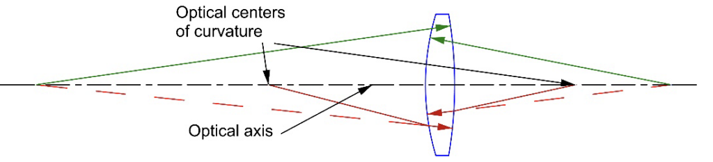
For a singlet optical element, the definition is simple. The optical axis is the line joining the centers of curvature of the two surfaces. The green arrows in Fig. 1 start at the physical centers of curvature. The red solid arrows start on the optical axis at the optical centers of curvature, that is, the position along the optical axis where the center of curvature appears located due to refraction at the intervening surface when viewed with an autostigmatic microscope (ASM) or an alignment telescope (AT). We will look at the process of using either of these instruments in a subsequent chapter. For now, we are just dealing with the definition.

Fig. 1 Physical and optical centers of curvature that define the optical axis of a single lens

We know one way of defining a line is with two points and those two points are uniquely defined here by the two centers of curvature as in Fig. 1. Independent of whether the surfaces are concave or convex, the optical axis is always normal at its intersection with the surfaces because the axis passes through the centers of curvature. This means here is no refraction or deviation of a ray propagating along the optical axis in either position or angle. This fact is implicit in the definition but seldom stated.

The definition shows why the optical axis is so important to alignment. When a lens is aligned to a reference axis and there is no deviation of a ray propagating along the reference axis the lens is perfectly aligned to the reference axis in tilt and decenter.

(Sidebar – There is a trap in this definition if you don’t think it all the way through. Say I have a lens and I want to center it in a collimated beam relative to some fiducial or datum perpendicular to the beam. I align my ASM or AT to the datum and insert the lens.  By tilting and decentering the lens I get the back focus well centered in my instrument. The image is well centered but by eye the lens looks tilted.

The trap is that I have tried to center the lens using the back focus only. That is a single point, so I only know 3 degrees of freedom (DOF) and I am trying to determine an axis, or a line. I need 4 DOF to do that. I do not have enough information to know the lens is centered, that is, whether the optical axis of the lens is parallel to the axis of the collimated beam. I need a second point such as the center of curvature of one of the surfaces to know the lens is completely centered.)

Optical axis of multiple elements

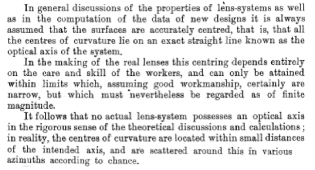
In looking for a definition of the optical axis of a real assembly of optical elements rather than the design of an assembly I stumbled upon this note by A. E. Conrady [1] from 1919 that states the situation I am discussing perfectly.

So, what is the “optical axis” of set of centers of curvature “scattered around…according to chance”? For the purposes of our discussion, I propose it is the analogue of the optical axis for a single element in a functional sense. What does the “scatter” do to the deviation of a ray propagating through the assembly? My definition is when the optical axis of an assembly of lenses is aligned to a reference axis an optical ray co-axial with the reference axis is not deviated in position or angle while passing through the lens. This begs the question of how we create a single optical ray, but we will get into that in another couple of Chapters.

The same trap occurs here as for the single element. When the system is aligned to the reference axis we must probe the transmitted ray at two distances from the lens to assure that neither the angle of the ray nor its position has changed. This aspect of the problem is getting ahead of myself, but I think you will agree that the definition makes sense assuming we can measure the transmitted ray.

Example of the optical axis definition for a “system” of elements

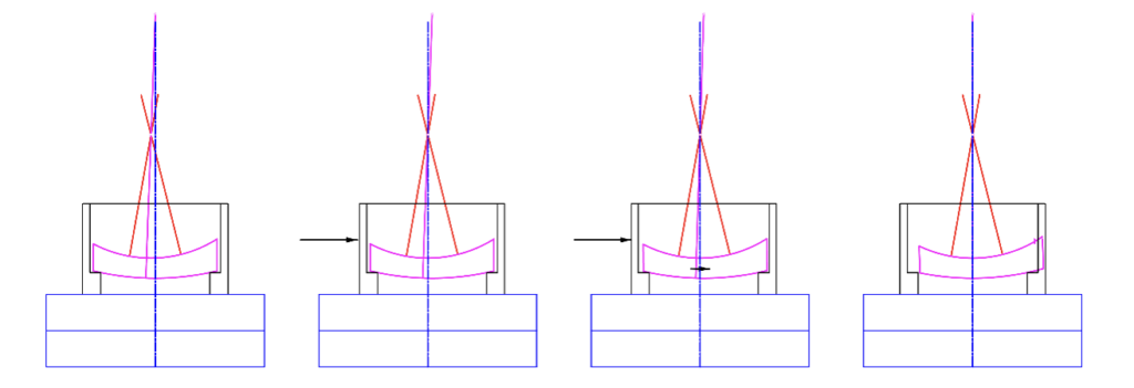
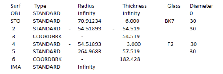
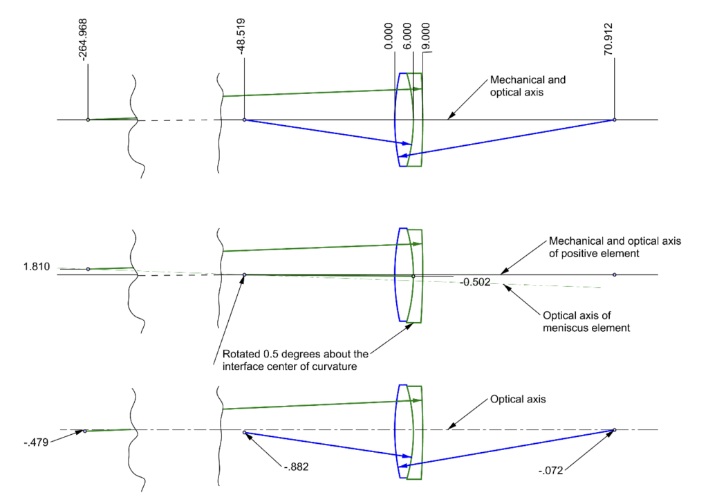
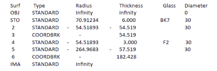
Consider a cemented doublet whose prescription is shown in Table 1. If the doublet is perfectly centered, the centers of curvature of all three surfaces lie on a straight line that is both the mechanical and optical axis as in Fig. 2a. If there is an error in cementing this is no longer the case. Assume there is a 30 minute of the meniscus relative to the positive element. This is about 10 times larger than the typical centering tolerance for an off the shelf doublet but the large decenter makes it possible to see the errors in Fig. 2

Table 1 Prescription of the cemented doublet used in the example

When the meniscus is rotated about the center of curvature of the 2nd surface of the positive element, the center of curvature of the 2nd surface of the meniscus moves 1.81 mm above the optical axis of the positive element. The mechanical vertex of the meniscus is about half a mm below the axis as seen in Fig. 2 (middle) 

To find the optical axis of this “system” the doublet is allowed to rotate and decenter about the 1st surface of the positive element relative to the initial optical axis of the perfectly centered doublet until the transmitted ray traveling along the initial axis in neither changed in position (ray height) or angle. A ray trace optimization program calculates the doublet must be rotated 0.389° CCW and decentered downward 0.553 mm for no deviation of the ray.

The correction places the centers of curvature of all 3 surfaces below the optical axis as in the lower part of Fig. 2. The centroid of the image formed at the back focus of the lens for a collimated beam parallel to the original axis would shift about 0.01 mm from the optical axis. Because a tilt about 10 times a typical tilt was used in the example, we get an idea of what to expect from a typical lens by scaling back a factor of 10. A 3 minute tilt is barely perceptible in most instances.

Throughout this discussion we have talked about using a single ray to establish the optical axis. Creating this single reference ray is discussed in a future Chapter.

Other definitions relating to alignment

Before talking about how to use optical instruments to align optics it is helpful to define a few more concepts. We will finish out this segment with these thoughts.

First, we have pointed out that a line, or axis, is defined by 2 points, or a point and 2 angles, 4 DOF altogether. Do not forget that a circle of any radius can be drawn through 2 points. To show 2 points lie on a straight line you need to measure a 3rd point and prove it lies on the same line.

Next, a plane mirror is a plane defined by 3 points, or 3 DOF. This is why you need 2 plane mirrors to turn an axis from one position and angle to another position and angle. There are not enough DOF to do it with one plane mirror. You need 4 DOF to define an axis. A good example are orthogonal galvo scan mirrors. You need 2 mirrors to scan over all angles in a hemisphere where the beam starts from a particular location and angle.

A spherical mirror or surface is defined by 3 DOF to determine the location of its center of curvature. You need a 4th point to know its radius of curvature. This is why when using a coordinate measuring machine (CMM), you need to touch the master ball in at least 4 places for the machine to know where the center of the ball is. This is the perfect example of a difference between optical and mechanical measurements, and why we can say that a spherical ball, or any part of a spherical surface, is an analog of a point. If a point source of light is at the center of a spherical surface the light will be perfectly reflected back on itself to the point independent of the radius of the spherical surface. 

For a mechanical measurement we need to also know the radius of the surface to know when the center of curvature is located. Not only do we need 4 points, but in the case of a concave mirror, 4 points around the edge won’t do. We need one point near the middle of the mirror to avoid an ill-conditioned situation that makes the calculation of the center of curvature a poor estimate. Further, most people do not like you to touch the middle of an optical surface. The safest method of finding the center of curvature of an optical surface is to do it optically. This is also the quickest and most precise method of finding the center of curvature.

This is why when using a coordinate measuring machine (CMM), you need to touch the master ball in at least 4 places for the machine to know where the center of the ball is. 

Cylinder – The next most complex surface is a cylinder that is defined by its axis, or 4 DOF. As an analog to a spherical surface, you can find the axis of a cylinder of any radius with 4 DOF, but you need a 5th point to determine the radius of curvature of the cylinder, just as you needed 3 DOF to find the center of curvature optically but a 4th point to find the radius. When a point source of light is focused at one of the axes of a cylinder the reflected light comes back to form a line image. Using an autostigmatic microscope you can find the axis in 3 DOF, 2 DOF in translation and 1 in angle.

Symmetric asphere – A symmetric asphere also requires (for alignment purposes) 4 DOF to define because as opposed to a spherical surface, a symmetrical asphere has an axis. A 5th point is required to define its vertex radius of curvature. We will get into more details about aspheres later but for now these are the basic alignment details.

Off-axis asphere and a toroid – An off-axis asphere requires 5 DOF with an addition point to define a radius in one direction. Toroids are included here because if you mask or stop down an off-axis asphere you effectively are left with a surface with 2 cylindrical surfaces of different radii at right angles to each other. There are cases where a toroid will be a satisfactory substitute for an off axis asphere just as a sphere can substitute for a symmetric asphere if the f/# of the surface is slow enough.

This is enough on definitions. In the next Chapter we will get into the first steps of classical alignment.

[1] Conrady, A. E. (1919). Lens-systems, decentered. Monthly Notices of the Royal Astronomical Society, Vol. 79, p. 384-39079, 384-390.

Chapter 4: Autostigmatic Microscope

There is no better way to describe an autostigmatic microscope (ASM) than to call it an autocollimator (AC) with a microscope objective attached to the front. This converts the AC from an instrument that measures 2 angular degrees of freedom (DOF) into an instrument that measures the location of the center of curvature of a spherical surface or wavefront in 3 DOF. 

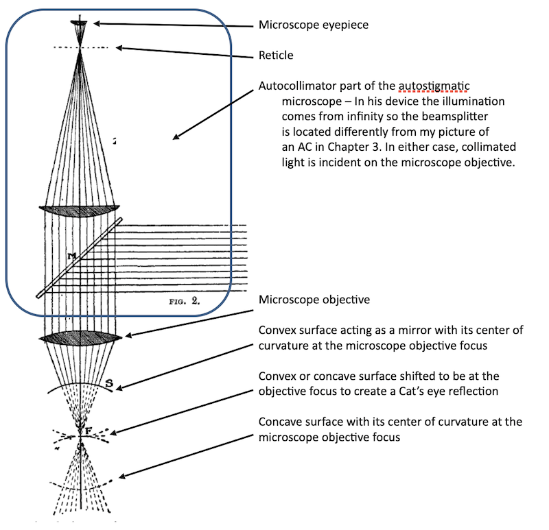
To illustrate this definition there is no better than the original description in the English literature, an article by a Mr. C. V. Drysdale in the Trans. Oct. Soc. London, 1900 called On a simple direct method of determining the curvatures of small lenses. In his introduction, Drysdale says he was surprised there was no instrument capable of measuring the radii of lens surface so “I immediately set to work to devise such a method, … capable of measuring the curvature of any spherical or cylindrical surfaces, from quite shallow curves to those of less than a millimeter radius.”

Drysdale’s Fig. 2 showed the method as reproduced here with my notes to the Figure.

opg chp 4 image 1

Although Drysdale’s original purpose was to measure radii of lens surfaces by first focusing at the center of curvature and then on the surface and measuring how far the microscope moved between the two measurements, he did not stop there. He went on to show his autostigmatic microscope could view aberrations in lenses by what we would now call the “Star test”, as well as measure object/image distances, focal lengths and principal plane locations. Suggested it could be used to measure index of refraction of glass and be used as a focimeter to aid optometrists.

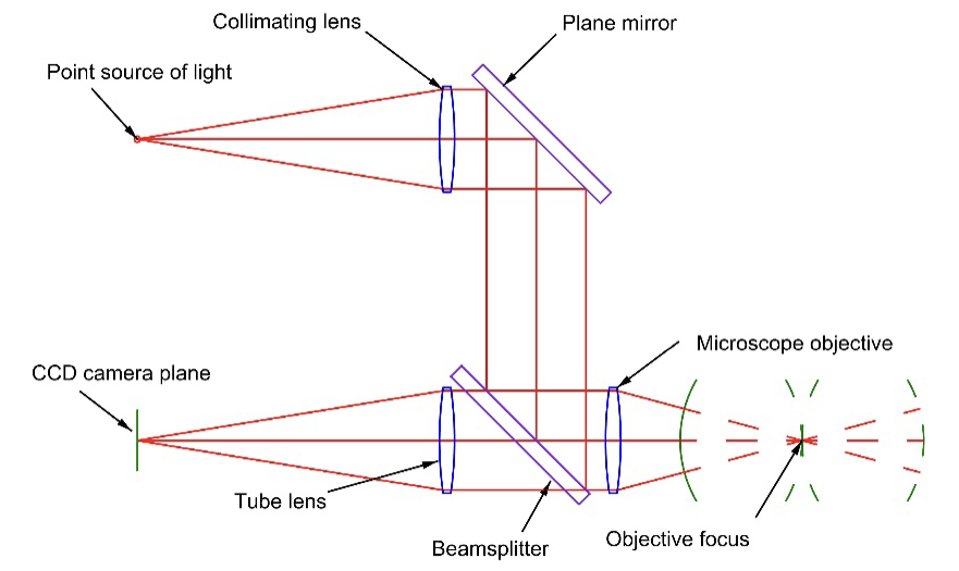
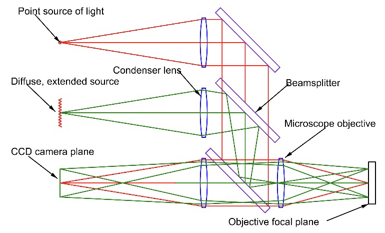
Modern ASMs have essentially the same optical layout as Drysdale’s and can do all he described and much more thanks to modern light sources and digital detectors. I will continue this discussion using the Point Source Microscope (PSM)* as the example of an ASM because I am most familiar with it and use it on an almost daily basis in my lab. The optical path in the PSM is shown in Fig. 1 when used as an ASM.

Fig. 1 The optical path in the Point Source Microscope when used as an ASM

While the optical paths are the same as in Drysdale’s paper, the light source is the free space end of a single mode optical fiber pigtailed to a laser diode at 640 nm to produce the smallest practical, but very bright, point source producing a near perfect spherical wavefront at the objective focus. In place of the eyepiece and user eye there is a digital camera with a 3.45 µm pixel, megapixel image in the ASM focal plane displayed on a monitor for convenient viewing and saving in a 16 bit format for post processing. At times we forget how much the laser and modern computer have changed optics. Most of the reasons the PSM can do more than Drysdale’s ASM is the vast range of controlled intensity of the source and the sensitivity range of the digital camera.

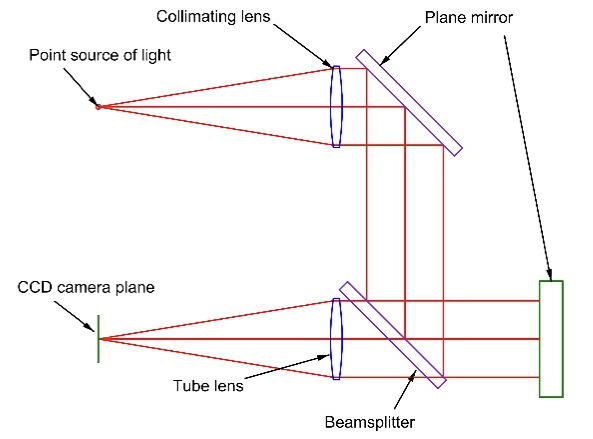
The PSM is also an autocollimator when the microscope objective is removed because of the collimated beam path inside as shown in the Fig. 2. Because the PSM has a shorter collimator, or tube lens, than most commercially available ACs, it has an angular sensitivity 3-4 times less but a larger angular field of view. This less angular sensitivity is a trade against the instrument size and mass.

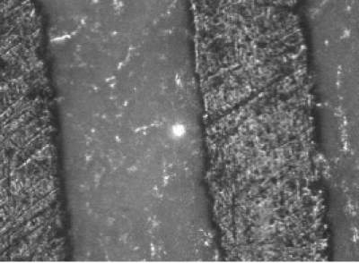
Although Drysdale does not mention it, his ASM had a feature that the PSM also has, it can be used as an ordinary reflection inspection microscope as in Fig. 3. There is a second light source in the PSM to give full field, nearly uniform illumination over a ~1 mm object space field of view (FOV) with a 10x microscope objective. This gives the option of locating a particular feature on a sample within the 1 mm FOV and illuminating a very small patch with an intense spot of light via the laser diode, or an external source fiber coupled into the PSM. Figure 4 gives an example of piece of paper with printed lines and the small bright image of the Cat’s eye reflection.

Fig. 2 PSM as an autocollimator

Fig. 3 PSM as an inspection microscope using diffuse illumination, and using the point source illumination

Fig. 4 Image of a 1 mm square area of a sample with a bright Cat’s eye reflection

Now that I have described an ASM and how it works I will discuss a few of the mechanical hardware tools used with the ASM and with autocollimators.

As mentioned earlier, an ASM locates a point in 3 degrees of translational freedom, but a point is an abstract idea. A solid, spherical ball is a physical realization of a point whose location is determined mechanically by touching its surface at 4 or more points to calculate its center. Because an ASM also finds the center of the ball to the same or better precision than it is found mechanically, the ball serves as an artifact that transfers an optical datum to a mechanical one, or vice versa.

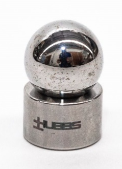
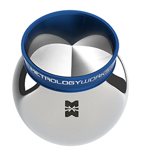
Steel balls are a perfect type of ball for this purpose. They are commodity items available in standard sizes and qualities. Half inch, 7/8” and 1.5” balls are particularly useful because these are the sizes of spherically mounted retroreflectors (SMR) and their mounts, or nests, used with laser trackers. Fig. 5 shows a 0.5” ball and nest while Fig. 6 shows a 0.5” SMR with a corner reflector mounted so its vertex is at the ball center. Because SMRs are mounted in spheres, an ASM is useful to locate them within a few µm of their required location.

 Fig. 5 ½” steel ball and nest designed to place the ball center ½” above the base

 Fig. 6 ½” Spherically Mounter Retroreflector. The cube corner apex is at the ball center

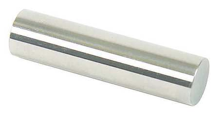
Pin or plug gauges are similar commodity items for use with an ASM, see Fig. 7. When the ASM is focused on the axis of the cylindrical gauge the reflection is a line image located in 2 translational and one angular DOFs. If the gauge is measured at 2 points along its axis, an ASM establishes the axis against which the plug gauge rests. Later is this series when we talk about alignment of asphere we show how plug gauges are useful datums for locating sagittal and tangential radii of curvature.

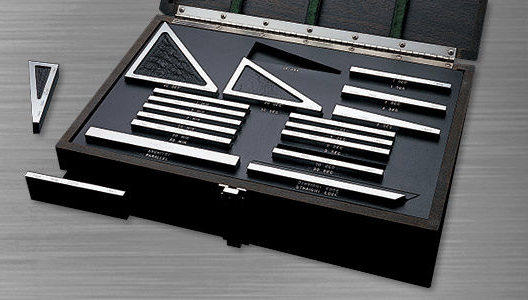
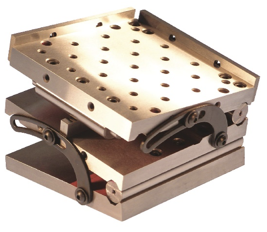
Obviously plane mirrors are useful with autocollimators. Aids in tilting plane mirrors are precision rotary tables and goniometers, sine plates and angular gauge blocks. See Figs. 8 and 9.  Sine plates and angle gauge blocks are relatively inexpensive methods of controlling angles to about 1 second of arc. Because you can use an angle gauge block in 2 directions, it only takes 9 gauge blocks to duplicate any angle between 0 and 90 degrees to 1 second of arc. Compound sine plates create 2 orthogonal angles by inserting standard gauge blocks between the platform and roll. 

Fig. 7 Plug gauge

Fig. 8 Set of angle gauge blocks

Fig. 9 Compound sine plate

To make an angle of 5°, for example, with a 10” sine plate you use a 0.872” gauge block because sin(5) = 0.08715.

Now that we have covered most of the hardware used to perform optical alignment we will move on to the definition of an optical axis and how to locate it for single elements as well as lens assemblies in the next Chapter.

*Full disclosure, my company, Optical Perspectives Group, LLC makes and sells the PSM.