Author: csadmin

Alignment Of Optical Systems

Written by csadmin on April 12, 2016. Posted in PSM Applications, Published Papers. No Comments on Alignment Of Optical Systems

1. Introduction

As optical systems become more complex and packaging requirements more severe and multi-dimensional, proper alignment becomes more challenging. Yet with current improvements in the manufacture and measurement of optical surfaces to nm levels, alignment is one of the few remaining opto-mechanical aspects of optical system manufacture and assembly where improvement in optical performance can be made. There are four approaches to aligning optical systems. These will be described and the advocated method illustrated by examples.

The preferred alignment method overcomes most of the difficulties of traditional methods but requires a new way of thinking about alignment. The method also requires alignment considerations must be studied immediately after the optical design is complete so that the necessary opto-mechanical datums can be incorporated into the mechanical design of the optical system cell, chassis or lens bench.

2. Methods of alignment

While one could argue with these definitions of alignment methods, they illustrate the point to be made. First is “snap together” or drop the elements into a cell which is the method traditionally used from the beginnings of centered optical systems. A cell and lenses are manufactured to tolerances governed by cost and performance considerations and then the lenses are set in the cell against their seats and held down by retainers. One then lives with the assembled performance of the system that is well modeled by Monte Carlo analysis. Since there will be a spectrum of performance outcomes in keeping with the model, optimum system performance will be achieved in only a few of these systems. However, this is the only economical method of assembling large volumes of optical systems.

Another method used on limited quantity, high performance, high cost systems is to assemble lenses into their seats while measuring each lens at its periphery for centration and vertex for spacing, and then testing the performance against a go/no go standard. If the performance falls below the acceptance criteria, the system is taken apart and reassembled as carefully as possible according to the design and tested again. This is a very tedious and costly procedure that exposes the optical components to many sources of damage through dis- and re-assembly.

A third method is a more systematic approach similar to the second but where the performance of the system is measured quantitatively in the pupil plane, possibly at a number of field points. If the system does not perform to an acceptable level optical design software is used to figure out what spacings and misalignments are causing the less than optimum performance, these adjustments are made and the system is tested again. Sometimes a second round of adjustments is necessary as changes in alignment affect performance non-linearly. While this method is more systematic it is still tedious and requires substantial careful testing and analysis of the test results.

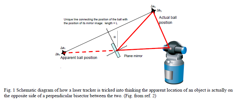
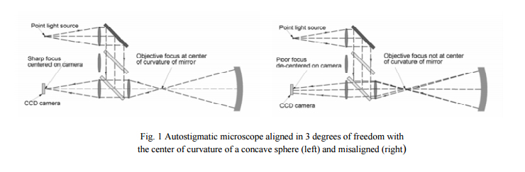
The fourth method that this paper advocates for high end, modest production systems is to locate the centers of curvature of each powered optical element at the exact design nominal location, or “true position” in mechanical engineering terms, and each plane mirror tilted and spaced so the beam focuses at the design nominal position after the fold. For centered systems this is most easily done by centering a datum seat in the cell on a rotary table and then checking that the light from the centers (or apparent centers) of curvature of the elements as they are assembled, one by one, do not nutate as the table is rotated as shown in Fig. 1.

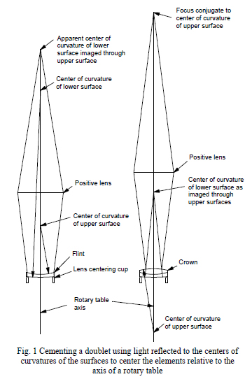
This example shows the cementing of a double where the flint element is placed in a centering cup and the cup centered until the reflection of a point source of light conjugate to the convex surface center of curvature (C of C) does not nutate. An auxiliary positive lens is needed to reach the apparent C of C but its focal length is not critical. The flint is then slid in the cup about the convex surface until the reflection of a point source of light at the C of C of the concave side remains still. The flint is then considered centered meaning that the line joining the centers of curvature of the two surfaces (the optical axis) is coincident with the axis of the rotary table. Then the lens is lightly clamped.

A drop of cement is placed in the concave well of the flint and the crown element is set in place. The concave surface of the flint now acts as an aligned centering cup so all that is needed is to make the reflection from the upper crown convex surface remain stationary. Again an auxiliary positive lens is required to access the C of C of the crown. The right hand side of Fig. 1 also shows how the apparent C of C of the flint has moved toward the lens due to the refraction of the crown.

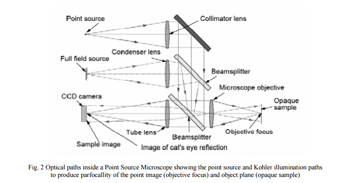
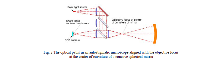
In this example we have referred to placing a point source of light at the C of C of a surface and then watching the behavior of the reflected image. The best way of doing this is with an autostigmatic microscope (ASM), a reflecting microscope with a beamsplitter behind objective and a point source of light produced by a single mode fiber located at the long conjugate of the objective. The return image can be viewed through an eyepiece or via a CCD camera. Fig. 2 shows a schematic illustration of the optical paths in a commercially available autostigmatic microscope.¹

3. Aligning two and three dimensional systems

Centered systems are a trivial case of locating C of C’s according to an optical design. Of far greater interest are two and three dimensional systems where the chief ray moves over a plane or in three dimensions. Since three dimensional systems are difficult to diagram successfully on paper, a two dimensional example will be given that amply illustrates the three dimensional nature of the problem. An imaging spectrometer from US Patent 6,288,781 by D. R. Lobb with powered prismatic elements is shown to scale in Fig. 3. Light enters a slit on the face of a plane prism at the upper left of Fig. 3. It passes through a prism with power on both the entrance and exit faces and proceeds on to an arrangement of three spherical mirrors similar to an Offner relay. The light exits through another prism with power on both surfaces to the detector plane.

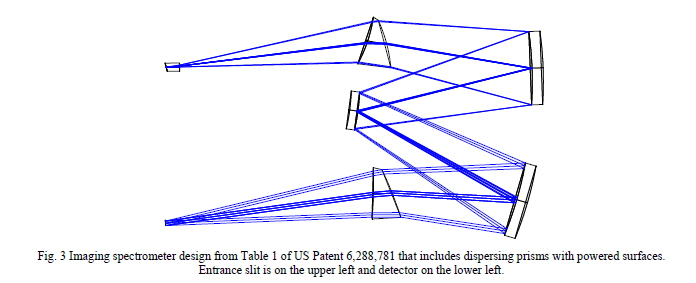
Fig. 4 shows the spectrometer in perspective and traces the chief ray from the entrance slit through the system to the middle of the detector plane. The line joining the entrance slit and detector plane is the axis of the spectrometer in an alignment, or opto-mechanical, sense just as the optical axis of a single refractive element is the line joining the C’s of C of the two surfaces. This axis defines five degrees of freedom of the spectrometer, three translations and two angles. We define the sixth degree of freedom in that we want the centers of all the elements to be the same height above a mounting plane.

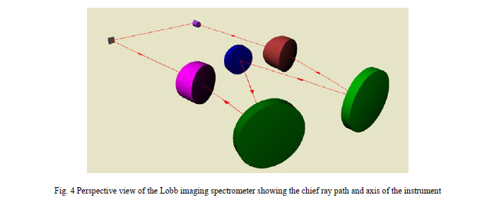
It is obvious that the edging tolerances and mount fabrication for the dispersing elements is going to be difficult as they will have to be located precisely and unambiguously in all six degrees of freedom relative to the spectrometer axis as defined by the slits. Of course the three mirrors also have to be properly aligned but this is a relatively simple matter compared to the prisms.

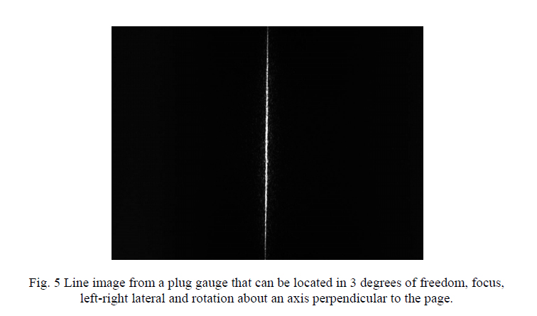
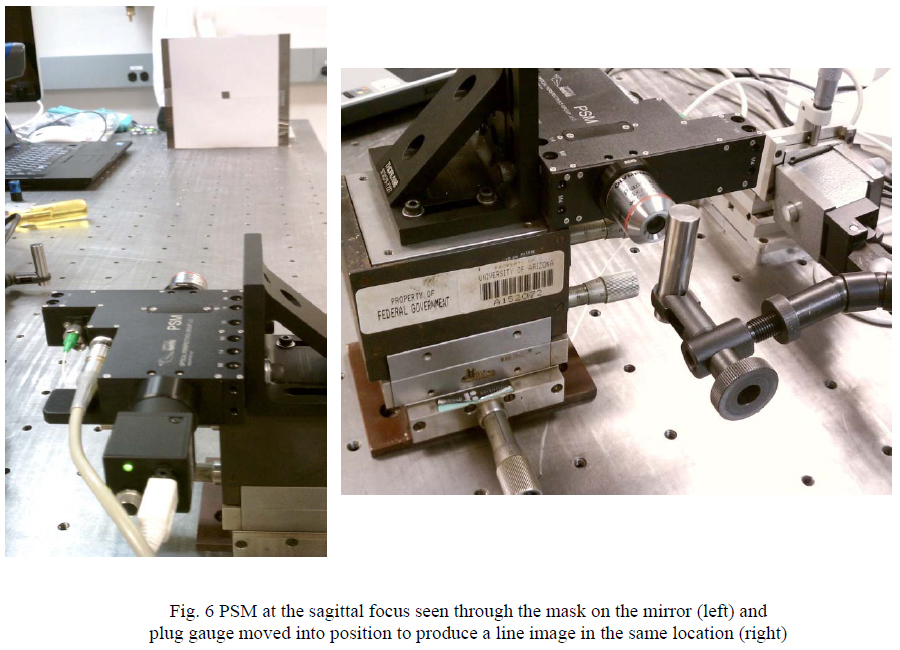
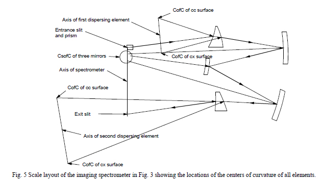
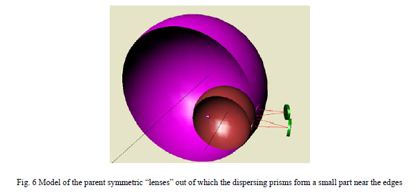
In order to accomplish this alignment we suggest that the next diagram to draw is the one in Fig. 5 where the C’s of C and axes of all the elements are located relative to the entrance slit and center of the detector, all in the plane of the paper. The centers of curvature of the three Offner relay mirrors are clustered together between the entrance and exits slits. Because the two centers of curvature of the dispersive elements each define three degrees of freedom, all six are defined for each element so they may be located precisely and unambiguously without reference to their edges. To illustrate where the dispersive elements lie relative to their axes we show the full elements in Fig. 6. This also illustrates why these elements would be difficult to fabricate without understanding their geometry. Once the geometry is understood the generating and polishing of the surfaces is not much more difficult than the surfaces of any lens.

4. Alignment of the system

In order to align the system a fixture is made either by drilling holes in the optical bench to which the elements of the spectrometer are mounted or in a fixture to which the optical bench is located by pins. In the holes a precision rod is placed with a conical hole in the upper end to serve as a mount for a bearing ball about 10 mm in diameter. A collar on the rod is used to locate the center of the ball to the height of the plane of centers of curvature. The rod and ball can be moved from hole to hole as one element is aligned after the other.

For the three convex surfaces, an auxiliary positive lens is needed to make the C’s of C accessible as already illustrated in Fig. 1. Holes and rods are also needed to support these auxiliary lenses but their locations need not be very precise as long as the lenses are centered on a normal to the convex surface that is roughly in the center of the surface.

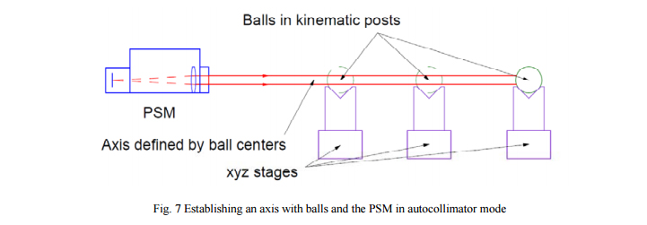
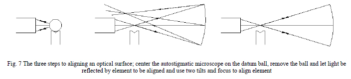
The short conjugate of the objective of an autostigmatic microscope is focused and centered on the center of the ball defining the C of C and pointing toward the element of interest. The ball is removed and the element adjusted until its center of curvature is focused and centered on the autostigmatic microscope display. Fig. 7 illustrates first aligning the autostigmatic microscope to the ball that defines the mechanical location of the C of C, removing the ball and aligning the mirror to the microscope. The microscope acts as the transfer device between the mechanical datum at the C of C and the optical surface. In the case of the refractive elements, having two microscopes makes this procedure much easier because both centers of curvature can be viewed simultaneously, one through the auxiliary lens. The order of alignment is governed only by avoiding the obstruction of the line of sight to the next surface.

When the alignment is complete a point source placed at the entrance slit will be well imaged at the detector. There can be no source of error unless the radii of the elements are substantially out of spec or the wrong glass was used. Since a good autostigmatic microscope can locate centers of curvature to < 1 μm, the translational errors of element locations can be held to about the same level and angular errors to a few seconds of arc (although the scale of the angular error will scale with the system size). The alignment is completely deterministic and does not depend on the type of optical system or even any knowledge of how the system will form an image because light is never put through the system the way it will be used during the alignment.

Alignment of folded systems with plane mirrors

Fold mirrors are plane mirrors used to change the direction of a beam of light and are useful in systems that must be made compact. If a light beam is focused it is defined by three degrees of freedom, the x,y,z coordinates of the focus. Since a plane is also defined by three points we have just enough degrees of freedom with two angles and one translation to change the beam direction and keep the distance from the last powered element to the focus constant. This does not count the two translational degrees of freedom needed to keep the beam centered on the plane mirror but these are not critical adjustments.

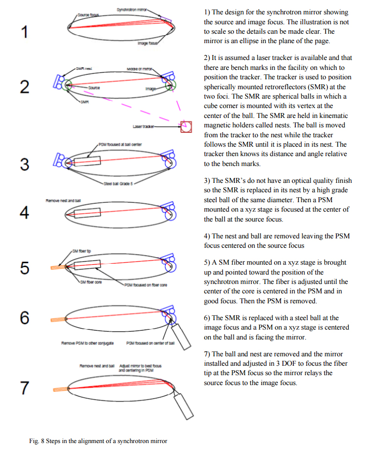
While we have been talking about folded systems the example we will use to illustrate the alignment of the plane mirrors was chosen to illustrate not only this section but the next concerning using aberration reduction as an alignment tool. Assume we want to put a deformable plane mirror in a telescope system for atmospheric error correction. This amounts to taking the beam of light coming toward the telescope focal plane and diverting it into a black box that corrects the wavefront and then spits the light back out so it focuses in the same place on the focal plane as it would have without the correction system. Whether the black box is in the system or not should be invisible to the detector. How do we align the fold mirrors to get the light in and out of the black box? A generic adaptive optical system (AOS) is shown in Fig. 8.

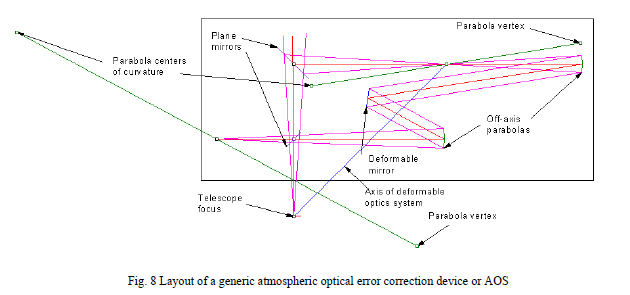
The AOS consists of a fold mirror to bend the beam headed toward the telescope focus to the entrance focus of the AOS, an off-axis parabola to collimate the beam, a deformable mirror to correct the wavefront, a second off-axis parabola to re-focus the beam and a final plane mirror to direct the output of the AOS to the telescope focus. If the whole optical bench were moved out of the way the focal plane would be none the wiser except the AOS decreases the f/number of the final beam somewhat. Just as in the imaging spectrometer we have identified an axis of the system with the sixth degree of freedom being the arbitrary angle about the axis.

For alignment purposes, the two plane mirrors must be precisely located so that the AOS does not appear to be in the telescope at all. To do this we first place a concave spherical mirror beyond the first fold mirror (mirror at top of Fig. 9) aligned so its center of curvature coincides with the telescope focus using an autostigmatic microscope (ASM) or similar device. Then we move the ASM so that it is focused at the center of the ball locating the exit focus of the AOS and is pointing toward the right. A second concave sphere is aligned to the microscope in tilt and focus.

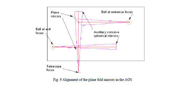
Then the microscope is moved back to the telescope focus as now defined by the concave sphere at the top and the plane mirror that folds the beam downward is inserted and adjusted in tilt and translation normal to its surface until the reflection from the concave sphere to the right is aligned on itself in the microscope. Now the microscope is focused on the ball at the entrance focus and is set to point toward the left. The entrance plane mirror is inserted and adjusted in three degrees of freedom until the return image from the concave mirror at the top is re-imaged on itself in tilt and focus. Now the plane mirrors are aligned to the telescope focus and the entrance and exit foci of the AOS. It now remains to align the powered optics of the AOS to the entrance and exit foci.

One aspect of this is to note that the alignment steps must be ordered so that no previously aligned optic interferes with the light path to another optic that needs aligning. This is why we had to use two concave spheres as tooling to align the two plane mirrors. Another aspect to note is that if the distances from the mirror to the foci are not equal it will not be possible to adjust the fold mirror so the chief ray follows the angle given in the design but will be incorrect by some angle dependent on the error in distances. This could come about in the design in Fig. 8 if the lens bench were incorrectly located too close or far from the focal plane. Then the exit fold mirror could still be adjusted so the output focus fell on the telescope focus but the chief ray of the AOS output would not be parallel to the chief ray from the telescope. In most cases a small error will not matter but it is something to be aware of.

Alignment using aberrations

Alignment using aberrations is very useful for locating optical elements with axes, particularly aspheric mirrors either symmetric or off-axis. While we will return to the AOS example momentarily, we give an example of where alignment using aberrations is sometimes seen in optical fabrication shops. The optician will want to test an objective lens with an interferometer for the transmitted wavefront quality. The test is so obvious that many fail to realize how sensitive the test can be to aberrations in the field and are surprised to see astigmatism and/or coma.

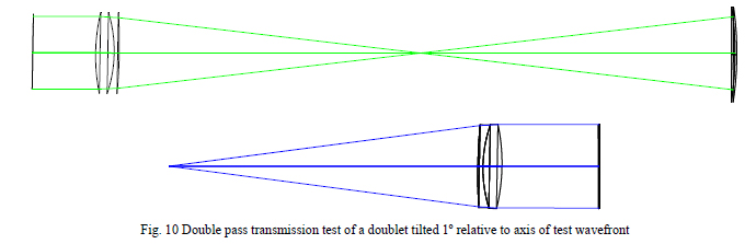
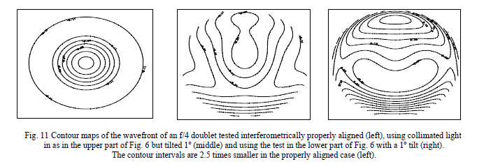
As an example, take a 25 mm diameter, f/4 cemented doublet. It can be tested interferometrically in either of two ways, collimated light in or focused light in against a flat, as shown in Fig. 10. Although it is not obvious without very careful examination the doublet is tilted 1º about an axis perpendicular to the page relative to the collimated beam from the interferometer (upper) or the return plane mirror (lower). Yet this misalignment that is not obvious without taking great care in the set up of the test yields substantial transmitted wavefront error that is not intrinsic to the doublet but rather due to its incorrect test. Contour maps of the wavefront aberrations are shown in Fig. 11.

This example is a simple demonstration of the importance of proper alignment to achieve full optical system design performance. Small alignment errors can have disastrous consequences on system performance yet be imperceptible without careful monitoring. This leads to the more interesting example of using aberrations for alignment. We will examine two cases, the alignment of a symmetric parabola to a flat (or collimated source) and the same example with an off-axis parabola to show there is fundamentally no difference in the approach.

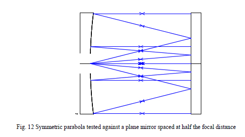
Assume we have a symmetric parabola with a central hole for the light to pass through. In this case a common test is to locate the test device focus at the mechanical center of the hole, let the out going light reflect off a flat placed at approximately half the focal distance from the parabola so the light fills the parabola and reflects back to the flat nearly collimated as shown in Fig. 12. The light then retraces itself back to the source when everything is aligned. The optical axis of the test setup is the line joining object and image and this we have located as soon as the image lies on top of the object, something easily seen with an ASM or when there are no tilt fringes in an interferometer.

The optical axis of the test set up must be aligned to the optical axis of the parabola for there to be no aberrations. The first step is to move the plane mirror longitudinally to focus the image and tilt the plane mirror until the object and image are coincident. If there is no coma then the parabola is perfectly aligned to the flat. In general this will not be the case. To finish the alignment the ASM focus (or the parabola) must be decentered in a direction to reduce the coma while the flat is tilted to keep object and image coincident. Moving the microscope in the direction of the point of the coma pattern will decrease the coma. Continue the decentering until the image is symmetrical. The location of the focus defines three degrees of freedom while the two tilts of the flat make up the balance of the five degrees of freedom needed for proper alignment. In this example with a 50 mm diameter, f/2 parabola just 23 μm of decenter (equivalent to 23 seconds in the field) will produce 0.1 waves of coma. This may be acceptable for viewing stars but is totally unacceptable for doing lithography.

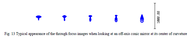
Going back now to the AOS where we talked about the positioning of the fold mirrors, there are also two off-axis parabolas that need aligning, see Fig. 8. The location of the focus of each has already been used in the fold mirror alignment. The vertices and C of C’s of these mirrors is also indicated in the Figure. If there is no indication of where the optical axis is on the off-axis mirrors the best approach is to put an ASM at the design location of the C of C of one of the mirrors and adjust the mirror to return the light into the ASM objective. As the mirror is moved longitudinally the combination of astigmatism and coma will produce an image that looks somewhat like a fish as shown in Fig. 13. The tail of the fish points toward the vertex of the off-axis segment.

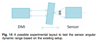
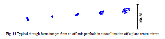
Once the off-axis mirror is located approximately correctly based on the location of its C of C an ASM is located at the design location of its focus and a plane mirror is used to reflect the nearly collimated light back into the off-axis mirror and ASM objective. The plane mirror should be used exclusively to get the light back into the ASM objective and centered on the display. Typical images might look like the through focus images in Fig. 14.

Adjustments should be made simultaneously to the off-axis parabola and the plane mirror to hold the image centered in the ASM and to orient the largely astigmatic image with the coordinate system, that is, make the astigmatism either horizontal or vertical. Once this is done tilt and decenter of the off-axis parabola and tilt of the mirror are only needed in one direction to shrink the image to a symmetrical, well focused image.² As the image approaches symmetry it may be necessary to touch up the alignment in the other direction as the astigmatism may rotate as the image symmetry and focus improve due to better alignment.

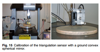
For the final example⁵ we take the single pass alignment of a convex secondary in an off-axis Ritchey-Chretien telescope as shown in Fig. 15. In this case we had already aligned the primary mirror and had collimated light entering the telescope parallel with the primary optical axis. The design indicated precisely where the system should focus relative to the primary vertex. The line between the primary focus and the system focus defined the optical axis of the telescope. The secondary axis had to be aligned to this axis in five degrees of freedom to eliminate any aberrations.

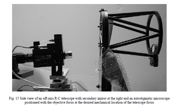
With collimated light entering from the right in Fig. 15 the primary and secondary mirrors brought the light to focus in the vicinity of the autostigmatic microscope objective focus. The microscope objective focus had been located via mechanical tooling (see Fig. 7) and does not move once located mechanically. The secondary is then adjusted in focus and either tilt or decenter until the focused light enters the objective and the badly aberrated spot is roughly centered on the viewing screen. When reasonably well focused light is centered in the microscope objective the secondary has been adjusted in three of the five necessary degrees of freedom.

It is then necessary to use a combination of tilt and decenter plus focus to hold the focused spot centered in the objective and to reduce the aberrations, now a combination of focus, astigmatism and coma. The procedure is exactly as described previously above. If the secondary mirror has five adjustment screws and a minimum of backlash it is possible to do the alignment in a matter of minutes.

Determining aberrations from images

It has been suggested that the alignment described in the above sections of the papers can be performed with an ASM or an interferometer. Except for one embodiment of a commercial interferometer (Fisba), interferometers are too large to conveniently adjust accurately and stably in five degrees of freedom, three degrees of translation with high resolution and two degrees of tilt to be sure apertures are approximately uniformly filled with light. Not only is an ASM easier to move conveniently and accurately adjust to the locations necessary for alignment, but the adjustments needed on the optics being aligned are easier to interpret from the image shapes than from interference fringes. Granted that low order aberration quantities can be read off the interferometer monitor and these used to guide adjustments, the hand/eye human interface using the image shapes tend to be more efficient. The only downside to using the image is that it doesn’t give quantitative results as to the aberrations although an ASM is sensitive to wavefront errors of less that λ/8. In this last section we will describe a simple means of extracting pseudo low order aberration content from the images viewed with an ASM.

Two dimensional images have five symmetries; there is a part of the image that does not vary with azimuth and this part corresponds to all the rotationally symmetric parts of an image such as focus, third order spherical and all the higher order spherical aberrations. There remain four symmetries that describe how the image changes when it is flipped left-to-right, top-to-bottom and both left-right and top-bottom^3,4. These are even-even and correspond to 3rd order and higher astigmatisms at 0º, odd-odd that are related to astigmatism at 45º, odd-even that are related to 3rd order and higher comas at 0º and even-odd relating to comas at 90 º.

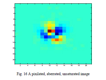
As an example take the image in Fig.16 where the pixels are 4.5 μm square and the image was magnified by a factor of 5 by the ASM. Because the region of interest around the image comprises relatively few pixels it is a quick calculation to find the even-even part of the image and then extract the rotationally symmetric part from that.

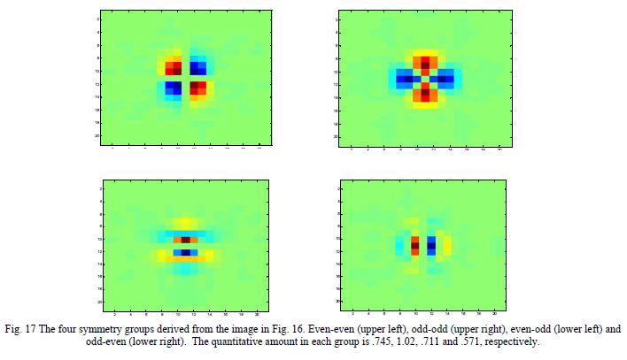
Once the rotationally symmetric part of the image is removed the image is further processed simply by flipping and adding or subtracting the flipped images to make four linear combinations of the original to form the four symmetry groups. Fig. 17 shows the four symmetries derived from the image in Fig. 16 after the rotationally symmetric part was removed. As is clear the four images bear a close resemblance to the two orientations of astigmatism and the two orientations of coma. While there are probably a number of ways to derive quantitative information on how big the proportions are of each symmetry type, we simply used the root sum square of the values at each pixel as the criterion.

Now as the alignment of an optical system becomes relatively good the pseudo aberrations derived from the symmetry of the image can be used to help determine the final adjustments of the alignment. Notice that this approach does not carry a sign for the pseudo aberration; all that can be done is to minimize each of the four aberrations. Also, some of the symmetry in the image will depend on how uniformly the pupil of the system is illuminated. Care should be exercised to make sure the ASM axis is well centered on the pupil of the system being aligned. The simplicity of the calculations makes it possible to update the results at TV frame rates.

5. Conclusions

The method of alignment by locating centers of curvature is a strictly deterministic approach to alignment that is particularly helpful for complex, folded and off-axis optical systems. Further, the method does not impose tight (read costly) tolerances on edging or mounts. The same principles can be applied to the alignment of plane, fold mirrors. Finally, using aberrations is an easy way of aligning aspheric optics. It is not presently widely used because the instrument to determine the aberrations is usually an interferometer and they are generally too large to bring to the optics in question. The ideal device to view images is an autostigmatic microscope and, until recently, there have been no commercial sources for these. Because the commercial ASM’s include software as an integral part of the instrument it is not difficult to derive quantitative values for the pseudo aberrations most useful for alignment.

If planning for this deterministic alignment method is incorporated in the opto-mechanical design of optical systems immediately following the lens design itself there need be no further acknowledgements such as the one that appeared in a recent paper about the design, fabrication and assembly of the ARIES imaging spectrometer used on the 6.5 m Multiple Mirror Telescope6, namely, “Thanks, Koby Smith, for banging your head against the wall to align the thing.” If alignment is approached in a logical and systematic manner as part of the opto-mechanical design from the outset of a project there is no need for anyone to bang their head against a wall.

6. References

¹R. E. Parks and W. P. Kuhn, “Optical alignment using the Point Source Microscope”, Proc. SPIE, 58770B, (2005).

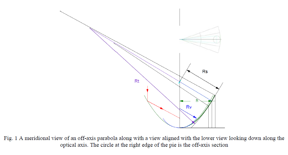
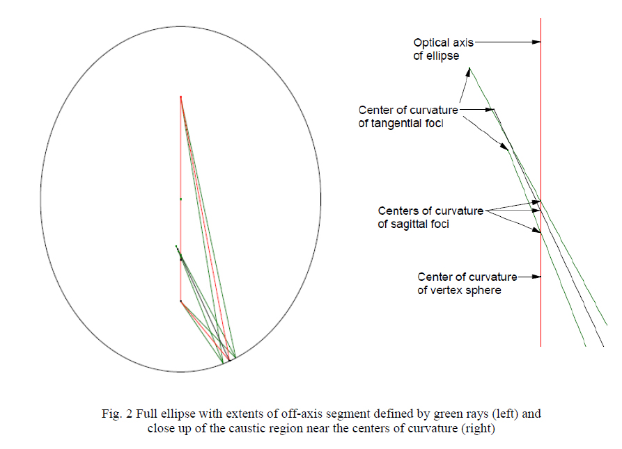
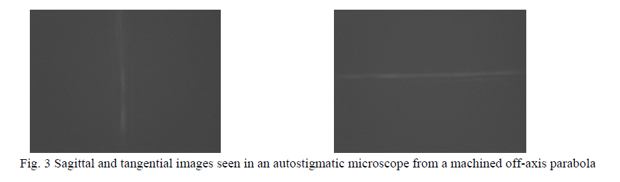
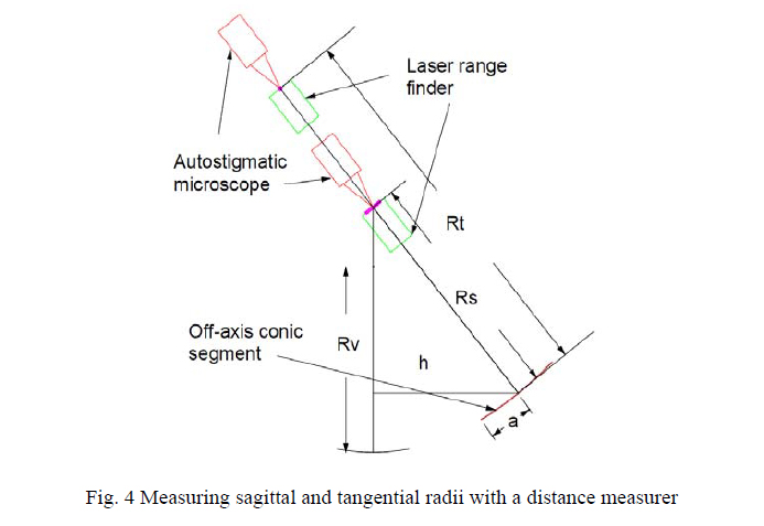
²R. E. Parks, “Alignment of off-axis conic mirrors”, Optical Fabrication and Testing Workshop Technical Notebook, OSA, Flamouth, MA Sept. 1980, pp 139-45. A revised reprint is available at ~~https://www.optiper.com/alignment%20of%20off-axis%20conic%20mirrors.pdf.~~

³C. Ai, L. Shao and R. E. Parks, “Absolute testing of flats(II); using odd and even functions”, Optical Fabrication and Testing Workshop Technical Notebook, OSA, Boston, MA 1992.

⁴C. Ai and J. C. Wyant, “Absolute testing of flats using even and odd functions,” Appl. Opt. 32, 4698- (1993)

⁵Work performed in collaboration with Breault Research Organization, Tucson, AZ.

⁶R. J. Sarlot and D. W. McCarthy, “A Cryogenic, 1-5 Micron Atmospheric Dispersion Corrector for Astronomical Adaptive Optics,” in Current Developments in Lens Design and Optical Engineering II, R. E. Fischer, R. B. Johnson, W. J. Smith, eds., Proc. SPIE 72, 4441 (2001).

Using The Point Source Microscope (PSM) To Find Conjugates Of Parabolic And Elliptical Off-axis Mirrors

Written by csadmin on April 12, 2016. Posted in PSM Applications, Published Papers. No Comments on Using The Point Source Microscope (PSM) To Find Conjugates Of Parabolic And Elliptical Off-axis Mirrors

ABSTRACT

Although the PSM is primarily an alignment instrument, it can also be used to determine the conjugates of parabolic and elliptical off-axis mirrors. By positioning the PSM at the sagittal and tangential foci of the mirrors, the conjugate distances of the mirror can be found using a laser range finder, for example. Knowing the sagittal and tangential radii of curvature (Rs and Rt), the vertex radius (Rv) is easily calculated. This information is used to verify that the mirror has been correctly manufactured and to aid in positioning the mirror in an optical system. Examples are shown of these steps.

1. INTRODUCTION

The alignment of off-axis aspheres is a subject that few people want to address because it is so different than aligning symmetric optics. An off-axis asphere has an optical axis, as opposed to a sphere that has no optical axis, just a center of curvature. Furthermore, the optical axis of the off-axis asphere usually does not pass through the surface of the mirror and certainly is not parallel to the normal to the surface at the center of the off-axis segment. On the other hand, off-axis aspheres are extraordinarily useful for many optical designs, and familiarity with them is essential for many optical systems.

This paper is an attempt to take some of the mystery out of off-axis parabolas and ellipses in terms of their geometry, and how to use their geometry to aid in their alignment. We will start by discussing some of the geometry that makes off-axis mirrors unique, and then describe how to find and measure the conjugates that are analogues to the center of curvature for a sphere. As opposed to a sphere with a center of curvature, an off axis asphere has two conjugates that define its axis, the two astigmatic foci at the centers of curvature of the tangential and sagittal radii of curvature. With the knowledge of how to find these conjugates, and a method of measuring the radii of curvature, it is possible to see that the mirror was manufactured correctly, and to see how the mirror should be aligned into the optical system for which it is intended.

2. GEOMETRY OF AN OFF-AXIS PARABOLA

Fig. 1 is a scale drawing of an off-axis parabola looking at a meridional section and along the optical axis (black vertical line). The off-axis section is the circle at the right edge of the pie section looking along the optical axis. It is aligned with the three vertical lines that defined the inner and out meridional extents of the off-axis section. The parent parabola is green and the blue circle has a radius equal to the vertex radius of the parabola while the purple circle segment, whose tangential radius is labeled Rt, is the best fit circle to the center of the off-axis segment. The light blue rays stopping at the optical axis define the sagittal radius of curvature, Rs.

The three radii are related by Rt = Rs^3/Rv^2 which makes it easy to find an unknown radius if the other two are known1. If a point source of light is placed on the axis of the parabola, a line image will form at the axis (light blue line perpendicular to the Rs ray). In general, the image will not be a line until the aperture of the off-axis section is masked, or stopped, down to a diameter where the coma in the off-axis asphere does not affect the astigmatism. How big a hole in the mask can be determined empirically, or an estimate of the coma may be made referring to Ref. 2.When the point source of light and the return line image are superimposed, the point source is on the normal to the surface at the center of the hole in the mask. The distance from the surface to the point source/line image is the sagittal radius, Rt. The astigmatic line image will lie in the meridional plane and is helpful in determining the azimuth of the vertex of the offaxis segment as well as determining the sagittal radius.

If the point source of light is moved back along the normal until the astigmatic line image is in focus it will be seen to be perpendicular to the meridional plane. The distance from the point source/line image here is the tangential radius, Rt. Since Rs = sqrt(Rv^2 + h^2) where h is the off-axis distance it is easy to find h.

3. GEOMETRY OF AN OFF-AXIS ELLIPSE

The geometry of an off-axis ellipse is a little more complex but the same basic geometry applies. Fig. 2 is a scale drawing of one of the parts we actually measured using the PSM and FARO arm. The green rays show the extent of the off-axis section relative to the foci to give a feel for the scale. The rays that bisect the rays going to the foci are those seen from the center of curvature of the off-axis segment. The right side of Fig. 2 shows the caustic region to give a better idea of the locations of the sagittal and tangential centers of curvature relative to the center of curvature of the vertex sphere.

As with the parabola, the sagittal foci lie on the axis of symmetry, or optical axis, while the tangential foci lie of the far side of the axis. From the way an ellipse focuses light from one focus to the other, we know the normal to the surface is the perpendicular bisector of the rays between the foci as shown. Just as with the parabola, we can find Rs and Rt, and using these values we can find Rv = (Rs^3/Rt)^1/2. For the ellipse we still need to find the conic constant, k, and the distance off-axis, h. To do this we make a mask as in the case of the parabola and measure Rs and Rt at 2 or 3 locations, h and ±delta h, where delta h is known. Two measurements will give an exact solution, while 3 or more will give a least squares solution using the relation that Rv^2 –k*h^2-Rs^2 = 01. The simplest method is to use 2 measurements at either edge of the off-axis ellipse and find the solution using the quadratic equation. One thing to remember is that delta h measured off the optic will be larger than it actually is, the distance from the axis of symmetry. Entering delta h as 1.4x less than the width of the optic is probably a good guess for a start.

Clearly with a concave ellipse this approach will get you close because the foci have to lie on the same line, the optical axis, as the sagittal foci. Also, for any given h, the line joining Rs and Rt lies on the normal to the surface. This will help locate the foci approximately. With this information it is then more precise to try to find the foci directly using the information derived from Rs and Rt. Using a point source such as the end of a single mode fiber at one focus and a microscope at the other focus it should be possible to locate the 2 foci to the precision necessary to meet system tolerances.

4. MEASURING THE SAGITTAL AND TANGENTIAL RADII

Using an autostigmatic microscope such as the PSM3, point the microscope at the mirror and locate the return image. Once the microscope is adjusted so the reflected point source is centered on the objective, focus the microscope to find either the sagittal or tangential focus. In general the reflected image will be too blurred to find a clean line image. Mask the mirror with an aperture small enough to produce a line return image. Adjust focus to get clean looking images such as that in Fig. 3.

When the microscope is well focused, bring a distance measuring device such as a laser distance measurer, or laser range finder4, up in front of the microscope and position it axially to get a focused Cat’s eye reflection off the rear of the distance measurer. Then take a distance reading to the mirror through the hole in the mask. Since most distance measurers calculate the distance from the rear surface of the instrument, the measurer reading is the sagittal or tangential radius, depending on which image is in focus. Fig. 4 shows how the measurement is made schematically.

Once these measurements have been made, the results may be compared with the prescriptions for the off-axis segments to see if the manufactured mirrors are to specification using the equations in the first part of the paper. It turned out in our case that one mirror was in spec and the other was not. Luckily it turned out that the specification was tighter than it needed to be and the mirror did not limit the performance of the system.

5. USE OF THE SAGITTAL AND TANGENTIAL FOCI FOR ALIGNMENT

There are at least two ways the focus information can be used for the alignment of off-axis mirrors. First, the measurements can be used directly by adding alignment features to the optical bench that the mirrors will be installed in. Since the two foci produce line images in reflection, we can use polished cylindrical artifacts to simulate the line foci. An inexpensive source of suitable artifacts are “plug gauges”5, cylinders about 50 mm long in diameters ranging from <1 mm to 25 mm or more. These are used the same way polished balls are as physical realizations of points to focus a PSM on, but in this case the cylinders are realizations of lines. Kinematic mounts should be made so 2 plug gauges are positioned where the sagittal and tangential foci are supposed to be located in the finished mirror system.

To align an off-axis segment, a PSM is focused on the line image formed at the axis of the plug gauge, the gauge is removed and the mirror adjusted so its focus appears in the same location as the line formed by the plug gauge. Fig. 5 shows a typical image on reflection from a plug gauge. The mirror can be located in 3 degrees of freedom, axially, one degree of translation, and one degree of rotation about the normal to the mirror surface. Once one focus is adjusted, the PSM is moved to the second plug gauge, and focused on it. The gauge is removed and the mirror adjusted by rotating around the first focus until second focus is correctly positioned laterally. This process may take some iteration because it may be difficult to make the mirror rotate around the first focus although with sufficient forethought the mirror mount could be designed with this adjustment built in.

A second method of alignment, an indirect one, is what we did. We located plug gauges at the two foci and then measured the locations of the gauges relative to fiducials on the mirrors. Fig. 6 shows how a plug gauge was adjusted to be at the same location as the line image formed by the mirror sagittal focus, in this case. This meant that when the mirrors were installed in their optical bench using the fiducials around the edges of the mirrors, we were effectively positioning the foci to their correct positions in space.

6. RESULTS OF MEASUREMENTS ON AN OFF-AXIS MIRRORS

The mirrors we measured were about 250 mm square and CNC machined out of 6061-T6 aluminum and then smoothed and polished by hand to a specular surface. One of the mirrors is seen behind the mask in the left hand part of Fig. 6. The ultimate use did not require the polish as they are to go in a terahertz wavelength (857 μm) radio telescope. On the other hand, we wanted to be sure the mirrors were sufficiently good to meet the telescope spec, and had been correctly machined and not deformed by the polishing.

Following the procedure described above we got the results shown in Tables 1 and 2. The standard deviation in terms of setting at the best focus of the line focus was about ±4 mm for the parabola and ±10 mm for the ellipse. The distance measuring laser gauge gave consistent readings within ±1 mm. Thus both mirrors had larger errors in their radii than could be attributed to measurement error. On the other hand, the radius errors amount to sag errors over the full aperture of 30 and 50 μm in the case of the ellipse, and 160 and 190 μm in the case of the parabola, compared with λ = 857 μm.

After reviewing these errors in manufacture in the optical design code it was felt that with a minor spacing adjustment the mirrors would work just fine as they were. This finding coupled with the knowledge of where the fiducials were relative to the radii of curvature meant that the system would perform as expected and could be successfully aligned.

7. CONCLUSION

We have shown how to determine the vertex radius of curvature and off-axis distance of off-axis parabolas by measuring the sagittal and tangential radii of curvature with an autostigmatic microscope such as the PSM. We have gone on to show how the conic constant may be determined as well by making multiple measurements of the radii of curvature for more general conics. This information is useful as part of incoming inspection to see if the optics ordered are the optics delivered. Further, we have shown how the locations of the radii of curvature can be used as a tool in aligning the offaxis mirrors into their optical systems using two different approaches to alignment.

REFERENCES

Smith, W., Modern Optical Engineering, 2nd Ed., McGraw-Hill, New York, 445-6 (1990)
Parks, R. E., Evans, C. J. and Shao, L., “Test of a slow off-axis parabola at its center of curvature”, Appl. Optics, 34, 7174-8 (1995).
See www.optiper.com
For example, see https://www.cpotools.com/bosch-dlr130k-digital-distance-measurerkit/ bshndlr130k,default,pd.html?start=1&cgid=bosch-locators-and-measurers
See, for example, https://www.mcmaster.com/#plug-gauges/=dbxtba

Method Of Alignment Using A Laser Tracker System

Written by csadmin on April 12, 2016. Posted in PSM Applications, Published Papers. No Comments on Method Of Alignment Using A Laser Tracker System

1. Introduction:

Laser trackers are an accurate and efficient tool for finding the locations of features in a threedimensional space but they rely on Spherically Mounted Retroreflectors (SMR) to return the laser beam to the tracker. If the feature cannot be contacted or it is not convenient to use an SMR another method must be used to follow the beam. We describe methods using a dual imaging and autostigmatic microscope for locating the features and two methods for tracking the microscope location depending on the type of tracker used. This converts a contact probe, large area CMM into a non-contact CMM by coupling a laser tracker with a dual purpose autostigmatic microscope. We begin with a brief description of the microscope followed by the alignment of the microscope to tracking and scanning laser metrology stations.

2. Point Source Microscope:

The imaging, autostigmatic microscope in question is called a Point Source Microscope (PSM)1 and has both a single mode fiber as a point source of light for the autostigmatic function and a LED behind a diffuser to provide Kohler illumination for imaging. The sources may be used independently or simultaneously. In the autostigmatic mode the PSM has lateral sensitivity of <1μm and similar axial sensitivity with an auxiliary lens for finding the centers of curvature of tooling balls or optics like mirrors and lenses. In the imaging mode the lateral sensitivity depends on the objective used but is in the neighborhood of a couple microns and the Cat’s eye reflection from a surface gives axial sensitivity to a similar resolution. It remains to show how to couple this non-contact ability to locate centers of curvature, the optically important feature of a lens or mirror for alignment purposes, to a high level of sensitivity to laser tracker systems that can determine locations in 3-dimensional space to similar sorts of accuracies.

3. Follower type laser tracking systems:

A follower type laser tracker is similar to a surveyor’s theodolite but is more sophisticated in that it is active. It sends out a laser beam along the telescope axis and the telescope will follow the beam if it is retroreflected back using a corner cube (generally a SMR that has the feature that the apex of the cube corner is accurately located at the center of the ball or spherical mount). The tracker will also measure distance using an interferometer mode if the SMR is moved from the tracker calibration SMR nest to a nest mounted on the measurand without breaking the laser beam. Fig. 1 shows how the follower tracker scheme works in general.

3.1 Alignment of the PSM to an SMR:

SMR’s are made in several convenient sizes, ½”, 7/8” and 1½” diameters, along with corresponding SMR “nests”, usually steel cones with a magnet at the apex to hold the SMR seated in the cone. A nest and corresponding SMR are mounted at a convenient location and the tracker is locked onto the SMR and its location in 3-D is noted. The SMR is removed from the nest and a grade 25 or better steel ball of the same diameter is placed in the nest so that its center is in the same location as the SMR. Then the PSM is adjusted so the focus of the objective is located at the ball center, something that can be done to <1μm in all three dimensions.

3.2 Alignment of the tracker to the PSM:

Attached to the PSM is a plate with a plane mirror in a mount that can be adjusted in tip, tilt and piston and a nest and an SMR. The plane mirror, shown schematically in Fig. 1, is nominally located half way between the objective focus and the SMR on the plate and perpendicular to a line between the focus and SMR. This arrangement is shown in Fig. 2. The mirror reflects the tracker laser beam back toward the SMR on the plate. The plane mirror is adjusted until the reflection from the SMR on the plate has the same apparent location as the SMR originally located at the PSM focus. The mirror is then adjusted such that the tracker sees the virtual image of the SMR at the objective focus. Now the assembly of PSM, plane mirror and SMR can be moved at a unit and the tracker will follow the PSM focus in all three dimensions as long as the PSM is not rotated so far that the tracker laser beam walks off the plane mirror.

4. Scanning type tracker system:

A scanning type tracker system uses several high speed rotating prism stations to sweep line images around a workspace. The prism scanners are accuracy synchronized with a clock. In the work space are detectors that resister when a beam sweeps by. Comparing the prism clocks and detector signals the detector locations can be accurately determined by time delay triangulation.

4.1 Alignment of the detectors to the PSM:

With the scanning system, three detectors are fastened to the side of the PSM facing two scanning prism stations. The PSM is focused on the center of a conveniently located steel ball. In this position the detectors are scanned by two scanning stations a known distance apart. Since three detectors on the PSM are scanned the plane of the detectors is determined relative to the scanning stations. The PSM with detectors attached is then moved to a different orientation while still being focused at the center of the ball and another set of data is taken to determine the plane of the detectors. This operation is repeated for a third orientation of the PSM while the PSM is centered on the ball. The three planes defined by the detectors will appear to rotate about the center of the ball, that is, a normal to each of the planes through the center of the ball are all equidistant as shown in Fig. 3.

This means the center of the ball, or focus of the objective, can be determined from the three measurements and once the distance from the center to the planes of the detectors is determined and recorded, any other position of the PSM can be related back to the center of the ball. This calibration is completely analogous to the initial use of a master ball and a touch probe on a Coordinate Measuring Machine (CMM) to establish the zero of the CMM coordinate system.

4.1.1 Using the calibrated PSM:

Once the center has been determined by this calibration, when the PSM is moved to any other location and the positions of the three detectors determined the location of the focus can be related to the center of the ball in all three coordinate directions. Any software that might be used with a CMM can also be used to analyze the data the scanner tracker gathers. This makes it possible to use the PSM precisely as a non-contacting probe with an apparent zero probe tip radius for any sort of coordinate measurements over large distances.

5.0 Conclusion:

We have shown how an autostigmatic microscope, and in particular, the Point Source Microscope (PSM) as a non-contact probe, can be used with laser tracker systems, either the follower type or the scanning type. In the first case an auxiliary mirror and tracker ball are used to make the tracker think it is looking at the focus of the PSM. In the second case, the PSM is calibrated in a way analogous to using the master ball on a CMM and then the PSM can be used as a zero radius probe tip for non-contact coordinate measurements over large distances. In both cases the PSM can be used either to find a center of curvature to 1 micron sensitivity in three dimensions or used in the imaging mode to locate a feature on a surface to 2 o3 microns in all three dimensions. The fact that the PSM images and can be set in all three coordinates to micron precision makes it a valuable part of an extension to contacting laser tracker systems.

6.0 References

1. Optical Perspectives Group, LLC, Tucson, AZ 85750, www.optiper.com.
2. J. Burge, et. al., Use of a commercial laser tracker for optical alignment, Proc. SPIE, 6676, 6676OE, (2007).

Swing Arm Optical Coordinate-Measuring Machine: High Precision Ground Aspheric Surfaces Using A Laser Triangulation Probe

Written by csadmin on March 10, 2016. Posted in Optical Testing, Published Papers. No Comments on Swing Arm Optical Coordinate-Measuring Machine: High Precision Ground Aspheric Surfaces Using A Laser Triangulation Probe

ABSTRACT

The swing arm optical coordinate-measuring machine (SOC), a profilometer with a distance measuring interferometric sensor for in situ measurement of the topography of aspheric surfaces, has shown a precision rivaling the full aperture interferometric test. To further increase optical manufacturing efficiency, we enhance the SOC with an optical laser triangulation sensor for measuring test surfaces in their ground state before polishing. The calibrated sensor has good linearity and is insensitive to the angular variations of the surfaces under testing. Sensor working parameters such as sensor tip location, projection beam angle, and measurement direction are calibrated and incorporated in the SOC data reduction software to relate the sensor readout with the test surface sag. Experimental results show that the SOC with the triangulation sensor can measure aspheric ground surfaces with an accuracy of 100 nm rms or better.

Subject terms: swing arm profilometer; profilometry; aspherics; optical testing; laser triangulation sensor; ground surface metrology.

Paper 120473 received Mar. 30, 2012; revised manuscript received May 16, 2012; accepted for publication May 30, 2012; published online Jul. 6, 2012.

1 Introduction

In the field of optical metrology for aspheric optics fabrication, most of the interferometric tests (visible spectrum range) that provide high-accuracy measurement are used after the test surface is polished. But at the polishing stage, the surface shape, or figure, correction is slow. It is desirable to measure the surface accurately during grinding to minimize figure errors and speed up fabrication.

Different techniques have been developed for testing ground surfaces. One traditional method is to use an infrared interferometer. However, as with visible interferometers, null optics are needed for measuring the aspheric shape. The design and alignment of the null optics are complex and time consuming. The limited infrared material choices and the nonvisible light make the use of the infrared interferometer even more difficult.

A laser tracker or laser tracker plus system¹ such as the one used for the Giant Magellan Telescope primary mirror segment is another way to measure a mirror during grinding. The basic idea uses a commercial laser tracker system with the spherically mounted retroreflector (SMR) touching the mirror surface. Since it is a point by point test, it takes time to collect a large number of samples.

There is a new prototype called SLOTS² based on reflection deflectometry using a long-wave infrared source scanning technique to measure the surface slope variation of ground surfaces. It is a simple, fast, low-cost, and non-null system that can measure surface slopes to microradian precision. The method is promising but needs further development.

The swing arm optical CMM (SOC),^3–5 developed at the University of Arizona, is a profilometer with a distance measuring interferometric sensor. It is used for in situ measurement of highly aspheric mirrors, and it has shown a performance rivaling full aperture interferometric tests. The interferometric sensor has high precision and a high data rate, but it only works for polished surfaces. A contact sensor, with a linear variable differential transformer (LVDT), has been used with the SOC to measure ground surfaces, but the measurement is time consuming, because the probe is picked up after each point to avoid scratching the surface.

Different types of sensors have been studied for ground surface metrology. There are some sensors based on the confocal principle⁶ with linearity at the submicron level. There are sensors based on laser triangulation that have a resolution of 10 nm and are insensitive to surface angular variation. The triangular sensors work on both polished and ground surfaces and were chosen and calibrated⁷ for use in our application. The laser triangulation technique has been used for many applications, such as inspection of free-form surfaces^8,9 and blind guidance.¹⁰ The measurement uncertainty due to speckle noise, the test lateral resolution, and the aspect of the test sensitivity to the surface texture distribution have been investigated.^11–13 For high-precision optical surface measurement applications like astronomical telescope mirror metrology, the only work reported are some simulations showing the potential measuring accuracy using different types of triangulation sensors.^14,15

This paper shows the results of calibrating a triangulation sensor and using it to measure large ground mirrors. The paper is organized as follows: In Sec. 2, we review the basic principle of the SOC and laser triangulation sensors. In Sec. 3, we describe the calibration of a triangulation sensor and show some metrology results compared to an interferometric null test of a highly aspheric mirror. Finally, conclusions are drawn in Sec. 4.

2 Principles

2.1 Principle of the SOC

The basic geometry of the swing-arm profilometer is shown in Fig. 1. A sensor is mounted at the end of an arm that swings across the optic under test such that the axis of rotation of the arm goes through the center of curvature of the optic. The arc defined by the sensor tip trajectory, for a constant sensor reading, lies on a spherical surface defined by this center of curvature. For measuring aspheric surfaces, the sensor that is aligned parallel to the normal to the optical surface at its vertex reads only the surface departure from spherical. The SOC uses this simple geometry with an optical, noncontact, interferometric sensor that measures continuously across the optic. The optic or test part is rotated in azimuth after each profile is measured. Figure 2 shows an example of the profiling pattern we generally use during a test. Since the arcs cross each other while the sensor scans the mirror edge to edge, we know the surface heights must be the same at these scan crossings. The crossing height information is used to stitch the profiles into a surface using a maximum likelihood reconstruction method.^3,16,17 Figure 3 shows the results of using the SOC and a full aperture interferometric null test to measure a 1.4-m diameter aspheric surface that has an aspheric departure of 300 μm. The SOC test shows excellent agreement with the interferometric test. The direct subtraction of the maps from the two methods, after alignment terms have been removed, shows a difference of only 9 nm rms, much of which appears to come from the interferometric test.

2.2 Principle of the Laser Triangulation Sensor

Laser triangulation is widely used in various applications to measure distances to objects. A common triangulation principle is to project a light spot on to the object and extract the distance information from the reflected or scattered light.¹⁴

High measuring rates, high spatial resolution, large measuring range, and zero applied force are significant advantages of the laser triangulation sensor over other types of distance measuring sensors.

There are two types of triangulation sensors normally used. The first one is an orthogonal sensor, in which the output plane is perpendicular to its optical axis. The second one has a tilted sensor, in which the output plane is tilted according to the Scheimpflug principle. Tilting of the output plane eliminates defocus and makes the sensor insensitive to the angular variations of the test surface due to the imaging effects.¹⁴ The sensor investigated and used on the SOC is the second type.

The geometry of the sensor measuring method is shown in Fig. 4. The incident beam with angle θ hits the surface at the sensor’s tip position O, where the sensor reads zero, and then reflects or scatters back and passes through an imaging lens inside the sensor. Finally, the beam falls on the detector of the sensor. The measuring axis is the bisector of the incident and reflected beam. By knowing the spot tip position and incident beam angle, we can trace the ray to O’ when the surface moves up to S2. The ray will reflect or scatter at the surface and be collected by the imaging lens if the distance d is within the sensor’s dynamic range. The sensor’s detector plane is tilted and is conjugate with the OO’ plane according to the Scheimpflug principle. The difference of the spot positions is a function of the displacement d, the projection beam angle, the magnification of the optical system, and the focal length of the imaging lens as described by Mikhlyaev.¹⁴ The commercial triangulation sensor is usually calibrated so that the output signal is linear with the test surface displacement.

3 Calibration

The sensor’s linearity, angular sensitivity, and scaling effect were measured experimentally. The zero position (tip position) of the sensor projected beam, the direction of the projected beam, and the measurement axis were calibrated and used as the input for the SOC data reduction. Finally, the system performance with the triangulation sensor was verified by measuring test surfaces with known shapes. The flow Fig. 1 Basic geometry of the swing-arm profilometer. chart in Fig. 5 shows the outline of the calibration steps.

3.1 Linearity

A distance measuring interferometer (DMI)¹⁸ was used to check the linearity of the triangulation sensor. The DMI has accuracy at nanometer level. The setup is shown in Fig. 6.

The DMI and the triangulation sensor were aligned to be able to measure simultaneously the motion from a double-sided flat mirror, which was mounted on a flexure. The flexure was driven with a voice coil and function generator to oscillate sinusoidally with a peak-valley motion of 2 mm at a frequency of a few Hz. One side of the double-sided flat mirror was specular as the target for the DMI, while the other side of the flat was ground for evaluating the triangulation sensor.

We budgeted a signal difference of 10 nm or less from the test system alignment and the motion effect. (The sensor has a 10 nm resolution.) The motion of the flexure with the flat mirror was designed and checked with an alignment telescope to show an angular variation of a few arc-seconds. The DMI and the triangulation sensor are aligned to each other to minimize the cosine errors and Abbe errors.

Figure 7 shows an example of the signals obtained from the DMI and the triangulation sensor.

The readout difference from the direct subtraction of the DMI and triangulation sensor data was ∼60 nm rms as shown in Fig. 8. The difference was dominated by the random noise from the environment and the ground mirror surface roughness, because the incident beam from the triangulation sensor moves across the mirror as it is oscillated. Later we show that when the sensor is mounted on SOC and tests a polished surface, a precision of 20 nm rms is achieved when an average of eight single measurements is used.

3.2 Calibration of the Geometry of the Sensor

3.2.1 Sensor tip location and the direction of the projected beam

When measuring a test surface, as seen in Fig. 9, the coordinates of the point of measurement are a function of the sensor position, the direction of the projected light beam relative to the surface, and the test surface shape. Following the SOC coordinate calibration concept described by Su et al.,4,5 we calibrated the relationship between the sensor nominal tip position when the sensor reads zero and the direction of the projected light beam relative to reference features on the sensor case, namely, three laser tracker spherically mounted retroreflectors (SMRs). When the sensor is installed on the SOC, the coordinate relationship is used to determine the sensor tip location and angle of the projected beam relative to the surface under testing. This is done by measuring the three SMRs’ locations with a laser tracker. Then at each scan position, the coordinates of the point of measurement on the test surface can be calculated with a simple ray tracing algorithm in the SOC data reduction code.

To perform the calibration, we used a point source microscope (PSM)¹⁹ and a laser tracker.²⁰ As shown in Fig. 10, a piece of 25-μm thick translucent shim stock was located between the sensor and the PSM. The shim stock was positioned normal to the sensor’s measuring axis. The sensor was mounted on an x, y, z stage that brought the sensor up to the shim stock until the sensor read zero. Then a PSM was brought up to focus on the backside of the shim stock, so the PSM was focused on the effective sensor measuring spot as seen through the shim stock. When the sensor and the PSM were in these positions, the locations of the three SMRs on the sensor were measured with the laser tracker. Then the sensor was moved out of the way, and the center of a solid steel ball was positioned at the focus of the PSM objective. Then the solid ball was removed from the SMR nest and replaced with an SMR.

The SMR was measured with the laser tracker as shown in Fig. 11. Now the laser tracker has information about the measuring spot location at the zero height reading of the sensor relative to the SMR nests on the sensor. By moving the shim stock to different sensor height locations of the projected beam and repeating the above procedures, several locations along the projected beam were measured, and the direction of the projection beam was determined. The thickness of the shim stock was backed out during the data processing. The accuracy of the calibration in terms of the SOC coordinates was determined to a few microns.

3.2.2 Sensor measurement axis

The readout of the sensor is the displacement d along the axis of the sensor as shown in Fig. 9. Thus it is important to calibrate the sensor measurement direction relative to the sensor axis and align the sensor axis to the SOC test system. This calibration was initially done using the setup in Fig. 6. After the DMI and the triangulation sensor were aligned to minimize the readout difference between the two sensors, we used a laser tracker to measure the three SMRs’ locations on the sensor. Then the double-sided flat mirror and the sensor were removed, and a reference flat mirror was put far from the DMI but normal to the DMI beam as shown in Fig. 12. We used a tracker ball touching the mirror surface to find the mirror surface normal. The sensor’s measuring axis was parallel to the DMI axis and the mirror surface normal. The projected angle θ shown in Fig. 6 can be calculated from these results and the direction of the projected beam.

3.3 Scaling Effect

A scaling factor is introduced if the sensor is tilted relative to the test surface. As seen from Eq. (1), the scaling factor can be derived from the triangulation sensor test geometry. The scaling sensitivity was tested by tilting the sensor relative to the double-sided flat as shown from Fig. 13.

In Fig. 13, θ is the beam projection angle, and φ is in the plane of rotation angle of the sensor. (The sensor readout is insensitive to the out-plane rotations for small angles.) This scaling effect needs to be taken into account during the SOC alignment to the test part. It has a sensitivity of ∼0.015∕ deg for the particular sensor we used. As the test surface aspheric departure gets larger, the scaling effect from the sensor angular alignment becomes more significant. For instance a test surface with a 2 mm peak-valley aspheric departure and with 0.01 deg alignment errors will have scaling induced errors up to 0.3 μm in P-V. This scaling sensitivity puts a long-term stability requirement on the SOC. The test triangulation sensor system is sensitive to the angular drift between the sensor and the test surface.

As seen from Eq. (1), the projection angle can also be checked by varying some known angles between the sensor and the double-sided mirror and then reading out the scaling factor from the difference between the sensor and the DMI readings.

3.4 Angular Dynamic Range

A large angular working range from the sensor is desired, as we would like the sensor to continue to work when the test surface normal is not parallel to the measurement axis of the sensor. This is the situation for the SOC when the surface has a large departure from a sphere or a flat. As seen from Fig. 9, we need to know the angular range over which the sensor reads out the surface sag d, independent of the slope of the surface. The triangulation sensor we are using has the property that the detector plane is conjugate with the testing location, which is along the line of the projected beam as shown in Fig. 4. Due to this imaging relationship, the sensor is insensitive to the local slope variations of the test surface.

A possible experiment layout for testing the sensor angular range based on the existing setup is shown in Fig. 14. However, the angular range of the DMI is only a few minutes of arc and cannot support the large angular range we would like to investigate.

Another approach might be using a wedged double-sided mirror. However, multiple samples would be needed for sampling the angular range we are interested in, and the sampling is not continuous.

Instead, we decided to test the angular range by measuring a ground optical surface with a known shape as described below. The results show that the sensor maintains good linearity over the angular range tested of about +?3 deg.

3.5 System Calibration

3.5.1 Calibration under a CMM with a ground spherical surface

The initial system test was done using a CMM as the scanning device before the sensor was verified for service on the SOC as shown in Fig. 15. The x and y linear stages of the CMM were used to scan and record the coordinates of the mirror under testing. (The coordinates were further corrected with ray tracing.) The CMM z axis was locked, and the surface sag was read out by the sensor. A spherical convex ground surface was measured for calibration. The radius of curvature and diameter of the sample mirror was chosen so that the 2 mm sensor working range and a 3 deg angular range could be checked by scanning the full aperture of the mirror.

The data were collected continuously along the x axis for different y values using the CMM. Figure 16 shows an example of the data obtained from the scans. Each line in the figure corresponds to a particular x scan with a fixed y value. This shows the sag value seen by the sensor relative to the angle between the sensor axis and the normal to the sphere being tested. The performance of the sensor for different working angles is checked by this sampling strategy.

The setup offered a simple way of collecting a large number of data points rather quickly. In addition, it was easy to calculate the theoretical sag of the sphere at each point to compare with the measured values. After removing the ideal spherical shape, the difference map in Fig. 17 shows an rms difference of 0.62 μm. The errors are dominated by the scanning errors from the CMM rails, the deflection of the sensor due to moments induced by the readout cable, and the ground surface roughness. No systematic errors due to sensor angular dynamic range issues were noticed.

3.5.2 Measuring an aspheric surface

To check the system performance, we attached the calibrated sensor to the SOC to guide the grinding of a 1-m diameter 80 μm P-V aspheric surface. Figure 18 shows the comparison of the measurements from the SOC and from a null interferometric test when the mirror was in its polishing stage. The results show the SOC and interferometer data agree with each other to 100 nm rms or better. This shows that the triangulation sensor is reliable for measuring both ground and polished surfaces.

4 Conclusion

The SOC is an important metrology technique for highly aspheric surface testing because of its versatility and high accuracy. It is configurable for measuring concave, convex, and plano surfaces. It can make in situ measurements, and its high-precision performance can rival full aperture interferometric tests. We have shown how the measurement range of the SOC can be extended to ground surfaces by using a calibrated laser triangulation sensor, and we have shown how to carry out that calibration. The experimental data show that the SOC equipped with a triangulation sensor can measure a test surface to a precision of better than 100 nm rms. This significantly improves the optical fabrication efficiency by extending precision metrology into the grinding cycle of the fabrication.

References

1. T. L. Zobrist et al., “Measurements of large optical surfaces with a laser tracker,” Proc. SPIE 7018, 70183U (2008).

2. T. Su et al., “Scanning long-wave optical test system: a new ground optical surface slope test system,” Proc. SPIE 8126, 81260E (2011).

3. P. Su et al., “Swing arm optical CMM for aspherics,” Proc. SPIE 7426, 74260J (2009).

4. P. Su et al., “Swing arm optical coordinate-measuring machine: modal estimation of systematic errors from dual probe shear measurements,” Opt. Eng. 51(4), 043604 (2012).

5. P. Su et al., “Swing arm Optical CMM: self calibration with dual probe shear test,” accepted to Proc. SPIE 8126, 81260W (2011).

6. Acuity laser measurement, “White light confocal displacement sensor,” 043604 (Nov 2010) https://doc.diytrade.com/docdvr/1391688/21942722/1308161289.pdf.

7. Keyence America, “High-speed, high-accuracy CCD laser displacement sensor,” Keyence America (2012) https://www.keyence.com/ products/measure/laser/lkg/lkg.php,
https://www.micro-epsilon.com/ displacement-position-sensors/laser-sensor/index.html.

8. N. Van Gestel et al., “A performance evaluation test for laser line scanners on CMMs,” Optic. Laser. Eng. 47, 336–342 (2009).

9. B. Muralikrishnan et al., “Dimensional metrology of bipolar fuel cell plates using laser spot triangulation probes,” Meas. Sci. Technol. 22, 075102 (2011).

10. J.-H. Wu et al., “The application of laser triangulation method on the blind guidance,” Proc. SPIE 8133, 81330V (2011).

11. R. G. Dorsch, G. Häusler, and J. M. Herrmann, “Laser triangulation: fundamental uncertainty in distance measurement,” Appl. Optic. 33, 1306–1314 (1994).

12. D. MacKinnon et al., “Lateral resolution challenges for triangulationbased three dimensional imaging systems,” Opt. Eng. 51, 021111 (2012).

13. M. Daneshpanah and K. Harding, “Surface sensitivity reduction in laser triangulation sensors,” Proc. SPIE 8133, 81330O (2011).

14. S. V. Mikhlyaev, “High-precision triangulation sensing of mirror surface,” Proc. SPIE 4416, 400–403 (2001).

15. S. V. Mikhlyaev, “Influence of a tilt of mirror surface on the measurement accuracy of laser triangulation rangefinder,” J. Phys. Conf. 48, 739–744 (2006).

16. P. Su et al., “Maximum likelihood estimation as a general method of combining sub-aperture data for interferometric testing,” Proc. SPIE 6342, 63421X (2007).

17. P. Su, J. H. Burge, and R. E. Parks, “Application of maximum likelihood reconstruction of sub-aperture data for measurement of large flat mirrors,” Appl. Optic. 49(1), 21–31 (2010).

18. Renishaw, “RLE system overview,” (2012) https://www.renishaw.com/ en/rle-system-overview–6594.

19. R. E. Parks and W. P. Kuhn, “Optical alignment using the point source microscope,” Proc. SPIE 5877, 58770B (2005).

20. J. H. Burge et al., “Use of a commercial laser tracker for optical alignment,” Proc. SPIE 6676, 66760E (2007).

Calculation Of The Vertex Radius Of An Off Axis Parabolic Surface Using The Sag Measured With A Three Ball Spherometer

Written by csadmin on March 9, 2016. Posted in Optical Testing, Published Papers. No Comments on Calculation Of The Vertex Radius Of An Off Axis Parabolic Surface Using The Sag Measured With A Three Ball Spherometer

Abstract

We describe a method of calculating the vertex radius of an off-axis parabolic segment using a three ball spherometer to measure the sag. The vertex radius is found by solving a set of six simultaneous, non-linear equations for the three coordinates of one of the ball centers and the corresponding three coordinates of the point of tangency of the ball with the surface.

1. Introduction

Three ball spherometers are the 1” micrometers of an optical shop and have been used for over 100 years to measure the radii of spherical surfaces.^1,2 The radius of curvature of a spherical surface can be calculated from a simple, three term formula that includes the measured sagitta, or sag, the distance from the central micrometer or indicator and the center of the balls and the radius of the balls.^3,4 Until recently, in spite of the simplicity of the formula that includes a square in one term, spherometers were sold with tables that converted sag readings into radii because optical shop personnel often did not have the skills or time to solve the formula. With the advent of pocket calculators it is now easy to solve the sag equation.

The sag equation is rather simple because the spherometer balls touch the surface at normals to the surface, and for a sphere these go through the center of curvature of the sphere and through the centers of the balls on the spherometer. In the case of an aspheric surface this is not so; the ball centers still lie on the normals to the aspheric surface but the normals do not go through the center of curvature of the asphere. The solution to this problem requires the solution of six non-linear, simultaneous equations, again something not easily undertaken even by rather mathematically adept optical engineers. However, with the advent of equation solvers such as the “Solver” function in Microsoft Excel, solution of these simultaneous equations is straight forward and fast. This is the problem we will illustrate.

2. Measured surface sag (T)

The measured sag, T, is the difference between the spherometer indicator reading when the spherometer is sitting on a plane surface, Fig. 1 (left), and when the spherometer is resting on the aspheric surface to be measured (right). We have shown the case for a convex surface but identical conditions hold for a concave surface with the exception that the sign of the indicator movement is opposite.

3. Geometry of the three ball spherometer

Referring to Figure 2, the spherometer has three balls on the points of an equilateral triangle. D is the diameter of the circle through the centers of the balls, S is the length of the side of the triangle and the distance between ball centers, P is the height of equilateral triangle, Ω the distance from the center of the triangle to the balls and r is the radius of the balls. B10 is the center of the ball located on the meridional plane of the parabolic segment and the vertex of the parabola lies above this ball. B20 and B30 are ball centers located symmetrically with respect to the meridional plane. Relationships of the sides of the spherometer are given below.

4. Geometry of the spherometer resting on the parabolic surface

We use a Cartesian coordinate system where z is the axis of symmetry of the paraboloid and y lies in the meridian plane. The origin is coincident with the vertex of the parent parabolic surface. When the spherometer is first set on the parabolic segment we place ball B10 on the meridional plane with the tip of the indicator approximately centered on the segment. At first we know only that X_B10 = 0, Y_B10 is approximately P less than the center of the segment and Z_B10 is r higher along the normal to the surface than where the ball touches the surface, Z_F10 = Y_B10^2/(2R_v) where R_v is the vertex radius of the parabola.

Referring to Fig. 3 we see the spherometer in two states, the final one (subscript 1) sitting on the surface and an initial one (subscript 0) where the calculation is begun. We start by assuming the plane of the three spherometer balls is perpendicular to the normal to the surface at F10. This allows us to calculate a starting position for B20, and by shifting the plane of the ball centers downward by r, the starting position for F20.

Then we assume the spherometer is iteratively rotated down to the surface about the center of B10. The point of contact, F10, will not change nor will the dimensions of the spherometer. However, as the spherometer is rotated so the other two balls rest on the surface the calculated dimensions of the spherometer will change. Since the spherometer dimensions cannot change we have a method of solution by simultaneously solving the six equations below for the centers and points of tangency of the floating balls.

5. Calculation of points of tangency to the parabolic surface of the equilateral triangle base

The six unknown variables are

and they are found by solving six equations simultaneously. The six equations are

The relationship of the ball center to the point of tangency along the normal to the surface

where α, β and γ are the angles of the normals to the surface at F21. Finally the distances between the balls

Once the six unknowns are found it is straight forward to find the coordinates of the center of the spherometer and project the indicator down to the surface of the parabolic segment normal to the plane of the ball centers. In general, the tip of the indicator will not hit the center of the segment exactly and a new value will have to be used for Y_B10 and the calculation repeated until the tip is close enough to the desired location. Notice too that we have calculated the sag assuming the vertex radius is correct. If the measured sag is different from the desired, the R_v in eq. 5 must be changed until the results match the measured sag.

6. Summary

We have shown how the sag of an off-axis parabolic segment as measured with a three ball spherometer may be used to determine the vertex radius of the segment. While this is not as easy as for a spherical surface, the calculation is well within the capabilities of an optical engineer with access to iterative equation solving software.

7. References

1. Grubb, H., Nature, 34, 85 (1886)

2. Ritchey, G. W., Smithsonian Contributions to Knowledge, 34 (1904)

3. Horne, D. F., “Optical Production Technology”, p. 324, Crane, Russak & Co., Inc., New York 1972

4. Malacala, D. “Optical Shop Testing”, p. 818, 3rd ed., Wiley-Interscience, 2007.

Practical Alignment Using An Autostigmatic Microscope

Written by csadmin on March 8, 2016. Posted in Centering, Published Papers. No Comments on Practical Alignment Using An Autostigmatic Microscope

ABSTRACT

Auto-stigmatic microscopes (ASM) are useful for bringing centers of curvatures of lenses and mirrors to the centers of balls used as part of an alignment fixture. However, setting up the fixture to get the balls used for alignment in a straight line to represent the optical axis generally requires another piece of equipment. We show that within a practical range, the autocollimation mode of a modern ASM can be used to align balls to an axis with about the same precision as they could be aligned with an alignment telescope, or laser tracker. As a lead in to this topic, we discuss our meaning of alignment, the means of positioning optically important features such as centers of curvature and foci to the coordinates specified on assembly drawings. Finally, we show a method of using an ASM along with other tooling to align a toroidal mirror using its foci.

1. INTRODUCTION

1.1 Definition of alignment

In a paper on alignment we should start by defining alignment. Every optical system is built to a design. First, there is the optical design, and it is used by a mechanical engineer to design a barrel or optical bench into which the lenses and mirrors are held. Throughout this design effort, the optical elements are assumed precisely located where the design specifies. It isn’t until the optical bench and elements come together that the issue of alignment comes up. It is at the assembly stage where the elements must be located precisely where the design or drawing specifies. This is alignment, getting optical features such as centers of curvature, axes, and foci positioned precisely as the design or drawing indicates.

In order to get the optical features located precisely, an instrument is needed that can sense the optical feature in question precisely. The same instrument, in conjunction with mechanical tooling, must also sense mechanical datums in the lens barrel or optical bench since the axes and foci of the optical system must be positioned precisely relative to specific mechanical features called out in the design. For example, the design may call for the optical axis of a system to be concentric with the outside of the cylindrical barrel of the assembly. Thus there must be a way of locating both the optical axis of the optical elements and the mechanical axis of the cylindrical barrel to assure coincidence of the axes.

1.2 Autostigmatic microscope

An instrument that can define both optical and mechanical datums in conjunction with some simple mechanical tooling is an autostigmatic microscope1 . In simplest terms, an autostigmatic microscope is a microscope that has a point source of illumination that is conjugate with a set of crosshairs in the image plane, either real physical crosshairs in an eyepiece or electronic crosshairs on a video display. If the autostigmatic microscope is perfectly aligned to the center of curvature of a sphere, the reflection from the sphere will form a well focused point image centered on the crosshair, that is, it defines 3 degrees of freedom (DOF). If the microscope is not well aligned the spot will be out of focus and shifted laterally from the crosshairs. Fig. 1 shows the typical optics of an autostigmatic microscope both aligned and misaligned with a concave sphere.

In order to make the autostigmatic microscope more useful, the addition of full field, or Kohler, illumination is helpful so the microscope can image as an ordinary microscope does. If the focal plane of the imaging arm and the autostigmatic focus are the same, the instrument is even more useful in that both types of illumination can be used simultaneously as will be illustrated in the first example of its use in section 2. A microscope with these features that is commercially available is called a Point Source Microscope2 and the optical paths in the microscope are shown in Fig. 2.

2. ALIGNMENT OF A STAGE COINCIDENT WITH AN AXIS OF ROTATION

2.1 Some definitions

As a first example of alignment with an autostigmatic microscope, we will consider the alignment of a single axis linear stage with the axis of a rotary bearing. The specific example will be a vertical stage over a rotary table used for centering lenses, but the example is just as applicable to the alignment of a lathe headstock with the lathe bed and tailstock center.

As with the term alignment, it is best to start with a definition or two. Since we are aligning an axis we should note that an axis is a line and a line is defined by two points, or a point and an angle in two planes, in other words by four DOF. Rotation about the axis and distance along the axis are not defined.

Another term used in conjunction with axes of rotation is centering and this can be confusing since there can be two meanings to centered. For a point, or spot, to be centered on an axis of rotation it is stationary when the axis is rotated. For the axis to be centered on the microscope, the axis must lie on the microscope axis, or crosshairs. The illustration in Fig. 3 helps explain the difference in the two concepts assuming a rotating table.

In the upper left of Fig. 3 the spots of light produced by the autostigmatic microscope move in a circle as the rotary table revolves about its axis. This means the light spot does not lie on the axis of rotation. In the lower left, the light spot is centered on the axis of rotation, but the axis of rotation is not centered on the microscope axis, or crosshairs. In contrast on the upper right, the spots are rotating about the microscope axis but are not centered on the axis of rotation, while in the lower right, the spots are both centered on the axis of rotation and that axis is centered on the microscope axis or crosshairs. In short, if the spots are moving in a circle, the spots are not centered on the axis of rotation meaning the center of curvature from which the spots are reflecting does not lie on the axis of rotation of the rotary table.

The same concept applies to centering an object in the microscope field of view. Consider the crosshair target in Fig. 4 that is imaged by the microscope. One end of the crosshair is indicated by a circle to show that the crosshair rotates as its center traces out a circle about the axis of rotation of the rotary table.

As seen in the lower left view of Fig. 4, the crosshair will rotate as the axis is rotated but the center of the crosshair remains stationary in the field of the microscope indicating that the crosshair lies on the axis of rotation but is not centered on the axis of the microscope while it is in the lower right view. The two types of centering require two physically different operations; to center the spots or crosshair on the axis of rotation, the optical surface must be translated or tilted relative to the axis of rotation. To get the axis of rotation to lie on the microscope axis either the microscope must be moved to the axis, or the axis of rotation translated or tilted to make it coincident with the microscope axis or crosshair.

2.2 Alignment of an axis

Now to the alignment of the vertical stage to the axis of the rotary table. Fig. 5 illustrates the situation. There is a rotary table in the lower part of the Figure and a vertical stage to the right. The Point Source Microscope (PSM) is shown in two positions on the stage, one focused on a target on the table using the imaging light source and one at the center of curvature of the plano concave lens lying on the table. These two foci of the PSM are the two points on the line defining the axis of the stage since the PSM is physically tied to the stage. The axis of the table is virtual because it cannot been seen, but it is made real by use of two simple fixtures, a crosshair target on the rotating table defining one point on the axis and the plano convex lens defining the other.

To align the axis of the rotary table to the axis of the stage as defined by the PSM focus, we must both make the target crosshair and the reflection from the concave surface stand still in space. This is accomplished by translating the target and lens, separately, relative to the table top. The target can be a piece of paper with the lens sitting on top. When the PSM in the imaging mode is focused on the paper the situation will typically look like the case in the upper left of Fig. 4. The target must be decentered relative to the rotary table top until it looks like the case in the lower left of Fig. 4. Then the target crosshair lies on the axis on the rotary table.

Similarly, at the center of curvature of the lens, the situation will look like the case in the upper left of Fig. 3 when the PSM is focused at the center of curvature using the autostigmatic mode. If the vertical stage is very decentered, the stage may have to be translated to get the return image in the field of view of the microscope, but the real task is to make the reflected spot cease to move as the table is rotated, that is, to achieve the case shown in the lower left of Fig. 3.

Once the crosshair and spot are centered, that is, not moving except in the case of the cross, rotating about the center of the cross, it is then necessary to translate and tilt the stage until the cross and spot both lie on the crosshairs in the microscope. When the alignment is finished the crosshair target will look like the case in the lower right of Fig. 4 and the spot will look like the lower right of Fig. 3. It is important to make these adjustments in the correct order, center the targets on the rotary axis first and then adjust the column. Further, remember that the target errors are seen doubled due to the rotation, and in the case of the spot, reflection. Do not try to make the full correction all at once. You will overshoot every time and the alignment will take at least twice the time it should. Make the adjustments in fractions of what it looks like the translation needs to be.

Notice, too, this alignment could not be done without some simple fixturing to “realize” datums that are virtual without the fixturing. In general, the most useful fixtures are spherical surfaces, physical realizations of points, and next most cylinders, realizations of lines. These make the most precise realizations because if lens surfaces or high grade spherical balls are used, their centers can be located to <1 μm. With images of crosshairs, it is difficult to use centroiding algorithms to achieve micron centering, but 10 μm centering is easy with images.

3. ESTABLISHING AN AXIS

In this example, we will describe how to use an infinity conjugate autostigmatic microscope to establish an axis. This is important because the majority of optical systems have a single axis of symmetry and alignment for these systems means having the centers of curvatures all lying on a common axis. In passing, the easiest way of establishing an axis is to use a good rotary bearing like in the previous example. However, there are many times when such a table is not available or the optics are too large to put on a rotary table.

For the alignment of a system with a single axis, fixtures or datums have to be positioned at precise locations along the axis. The lateral positions are tighter than the axial locations, but the axial locations still need to be carefully controlled. The most common way to do this alignment is with an alignment telescope3 , but it is a tedious proposition and almost always requires two people, one looking in the eyepiece and one making the adjustments to the fixtures.

There is an alternative that works well over distances from about 0.5 m to 3 m. That is, remove the objective from the autostigmatic microscope and use the collimated beam projected by the 6 mm aperture. When the collimated beam reflects off a spherical surface, the return wavefront is nearly spherical, and for that part of the wavefront returning through the aperture on the microscope it is perfectly spherical assuming a good grade spherical ball. This situation is like that shown in Fig. 6 where a steel ball is used to maximize the reflected light.

The spherical wavefront reflected off the ball will have a radius of curvature of approximately the distance from the microscope to the ball. Assume for this example the distance is 1 m and the ball is 25 mm in diameter. The PSM has a 6 mm aperture and a 100 mm tube lens. This means the return wavefront will produce a spot about 0.6 mm on the 1/3” CCD detector that is 3.6 mm in the short direction. While this is not a perfectly focused spot, the centroiding algorithm in the PSM software works just as well on out of focus images as well focused ones. The limit here is that the entire spot lie on the CCD. In this example, the shortest distance from ball to PSM would be 250 mm to keep the image from being bigger than the detector. If a shorter distance were needed, the 6 mm aperture could be stopped down. Also, short distances mean plenty of light gets back through the aperture stop.

The far distance is limited by the light available but has the advantage that the spot on the CCD is smaller. For the example, the 6 mm collimated beam is spread into a cone of 0.235 steradians. At a 1 m distance, the 6 mm aperture subtends just 36 μsteradians, or collects just 1.5×10-4 of the reflected light assuming a top hat intensity distribution. On the other hand, the PSM has an intensity dynamic range of about 1×105 . Thus a dynamic range at a distance of 3 m or more is perfectly reasonable.

Figure 7 shows the PSM used in the autocollimator mode to align a set of balls on a common axis. Here the farthest ball is aligned first. A post such as used to position lens mounts can be used as a kinematic locator for the ball. The post is on an xyz stage and the stage is adjusted until the reflection from the ball is centered on the PSM display. Subsequent balls are similarly adjusted. The axial spacing is set using an inside micrometer.

There are several advantages over using an alignment telescope in addition to those already mentioned. The collimated beam is bright enough to see under ambient lighting so it is easy to set up the initial alignment, the balls are easier to use than crosshair targets needed with an alignment telescope, the set up has no moving parts in the alignment instrument and there is nothing to focus. Finally, the centroiding is completely objective.

In terms of precision, the centroiding algorithm has a sensitivity of just under 1 arc second, or ~5 μradians. Even with out of focus images on the detector experience has shown this to be the case. The means that balls aligned using this method can be positioned to about ±5 microns at the distance of 1 m. Over the range where sufficient light reaches the detector this sort of precise is on the order of that achievable with a laser tracker.

4. ALIGNMENT OF SYNCHROTRON MIRRORS

The final example is one that I have not had the opportunity to try out but is illustrative of a technique that could be applied to many situations where high precision alignment is required in a multi-dimensional space. Further, it shows how the autostigmatic microscope can be used along with other sophisticated optical tooling such as a laser tracker4 to increase the value of both the tracker and the microscope. The whole example is laid out in Fig. 8 and the various steps will be described in the text, one after the other. This is again an example of how there is a particular sequence of steps that must be gone through to achieve the final alignment.

The synchrotron mirror is⁵ almost plane and thus has the same DOF as a plane mirror, rotation about the axes parallel to its face and translation perpendicular to its face. Using these 3 DOF the mirror is adjusted so the light from the fiber tip is focused at the PSM focus. The focus will be a line normal to the page and have a width limited by diffraction set by the apparent width of the mirror looking into it at grazing incidence in the plane of the page. The other 3 DOF are set using mechanical datums on the mirror and the structure holding the mirror.

In this example we have tried to demonstrate the use of the autostigmatic microscope with other optical tooling used in large optical projects. The SMR’s used by the laser tracker are completely compatible with the use of steel balls used in other autostigmatic microscope applications. The imaging aspect of the PSM permits its use in the location and centering of an optical fiber tip that will then be used as a point light source at one conjugate of the system. Finally, the PSM can be used to detect the focused image coming single pass through the optical system to align the synchrotron mirror.

5. CONCLUSIONS

We have first set out a working definition of optical alignment as determining the location of an optical, as opposed to a mechanical, feature, and then moving that feature to the location specified in the design of the optical system. Then we have given a simple example of the alignment of a center of curvature to an axis of rotation to show the difference between alignment of the feature to the axis of rotation, and the alignment of the axis to the instrument making the measurement. This is followed by an example of using an infinite conjugate autostigmatic microscope to align a series of spherical ball targets in a straight line. Finally, we show how to use an autostigmatic microscope in conjunction with a laser tracker to systematically align a synchrotron mirror using the mirror’s two foci.

REFERENCES

[1] Steel, W. H., “The Autostigmatic Microscope”, Optics and Lasers in Engineering 4(4), 217-227 (1983).
[2] www.optiper.com
[3] For example, https://www.brunson.us/p/AboutAlignTel.asp
[4] For example, https://www.faro.com/laser-tracker
[5] https://www.bnl.gov/nsls2/project/CDR/Ch_08_Radiation_Sources.pdf, p. 18.

Author: csadmin

Alignment Of Optical Systems

1. Introduction

2. Methods of alignment

3. Aligning two and three dimensional systems

4. Alignment of the system

5. Conclusions

6. References

Using The Point Source Microscope (PSM) To Find Conjugates Of Parabolic And Elliptical Off-axis Mirrors

ABSTRACT

1. INTRODUCTION

2. GEOMETRY OF AN OFF-AXIS PARABOLA

3. GEOMETRY OF AN OFF-AXIS ELLIPSE

4. MEASURING THE SAGITTAL AND TANGENTIAL RADII

5. USE OF THE SAGITTAL AND TANGENTIAL FOCI FOR ALIGNMENT

6. RESULTS OF MEASUREMENTS ON AN OFF-AXIS MIRRORS

7. CONCLUSION

REFERENCES

Method Of Alignment Using A Laser Tracker System

1. Introduction:

2. Point Source Microscope:

3. Follower type laser tracking systems:

4. Scanning type tracker system:

5.0 Conclusion:

6.0 References

Swing Arm Optical Coordinate-Measuring Machine: High Precision Ground Aspheric Surfaces Using A Laser Triangulation Probe

ABSTRACT

1 Introduction

2 Principles

3 Calibration

4 Conclusion

References

Calculation Of The Vertex Radius Of An Off Axis Parabolic Surface Using The Sag Measured With A Three Ball Spherometer

Abstract

1. Introduction

2. Measured surface sag (T)

3. Geometry of the three ball spherometer

4. Geometry of the spherometer resting on the parabolic surface

5. Calculation of points of tangency to the parabolic surface of the equilateral triangle base

6. Summary

7. References

Practical Alignment Using An Autostigmatic Microscope

ABSTRACT

1. INTRODUCTION

2. ALIGNMENT OF A STAGE COINCIDENT WITH AN AXIS OF ROTATION

3. ESTABLISHING AN AXIS

4. ALIGNMENT OF SYNCHROTRON MIRRORS

5. CONCLUSIONS

REFERENCES

USA

USA/INTERNATIONAL

UK & EU

All Asian Countries Except China

China

Australia & New Zealand

India