PHYSICAL RAY TRACING WITH BESSEL BEAMS

Authors: Robert E. Parks (Optical Perspectives Group, LLC) and Daewook Kim (J. C. Wyant College of Optical Sciences, University of Arizona).

INTRODUCTION

Following the discovery of so called non-diffracting Bessel beams[1], they have been used for a number of exotic purposes such as trapping single atoms and aiding in the discovery of exoplanets. We discuss more mundane but practical methods applicable to precision engineering, and the physical ray tracing of a ball lens in transmission to determine if it  behaves as geometrical optics predicts. 

First, we discuss the definition of a Bessel beam (BB) and how one is created [2]. Then we look at some of the BB properties to give the context of why they are valuable tools for tracing rays in the laboratory as opposed to mathematical ray tracing on a computer (i.e., non-realizable in practice due to the divergence of a very thin ray). We end by showing experimental results from using a BB to trace rays through a ball lens to show how well the experimental results match the computer paraxial ray trace of the same lens.

BESSEL BEAMS

A BB is simply a light intensity pattern in a plane perpendicular to its axis of propagation that is described by the  Bessel function, (J₀)². It has a bright central peak surrounded by rings of decreasing intensity. The beam core is non-diffracting in the sense that its diameter is much less than you can create with a collimated beam by any other means. The core of the beam is 100 to 1000 times smaller in diameter than the beam from a HeNe laser, for example.

In addition to being much smaller in diameter (i.e., spatially well-localized) than a laser beam, BBs are robust and less affected by air turbulance because they propagate through a larger volume of air which helps to average out the environmental effects [3].

One way of creating a BB is shining a collimated or spherical wavefront on a plane grating made of uniformly spaced concentric circles[4]. In practice today, such a grating is made by ebeam lithography on a photomask substrate with circle spacings on the order of 10 µm. It is particularly convenient to illuminate the grating with a point source of light made by the end of a single mode optical fiber pigtailed to a laser diode. The advantage over a collimated wavefront is that the length of the BB is much longer than with collimated illumination [5] and you do not need a good collimating lens the size of the grating. 

A disadvantage of point source illumination is that the central core of the BB expands as the beam propagates but the core maintains a peak intensity about 10 times that of first and subsequent surrounding rings. This means that the simplest sort of centroiding algorithm can still find the location of the core precisely.

PHYSICAL RAY TRACING

We know from simple geometry and lens design software that when a paraxial ray enters a lens at a known ray height and angle that it exits at  the same height but different angle at the principle plane. In 1996, Santarsiero showed theoretically that BB behaved as paraxial rays propagating thorough ABCD optical systems [6]. We show experimentally that when a BB is projected through a ball lens, the beam traverses the ball as though it was a single paraxial ray in a lens design program. 

Obviously, how the rays exits a lens will also depend on the intial alignment of the lens to a coordinate system. To avoid questions of alignment, we demonstrate physical ray tracing using a ball lens because such a lens cannot by misaligned in tilt. The only data of a ball lens are  its radius and physical center; its center of curvature. If the detector of the position of the BB is centered on the BB prior to inserting the ball lens in the beam and the ball lens is centered so the beam is again centered on the detector, the BB must be passing through the center of the lens and the lens is free of tilt since a sphere has no axis [7].

We show that the BB traverses the lens and continues to propagate in free space precisely as predicted by geometrical optics, and that the beam’s height and angle can be measured at any arbitrary distance along the axis of the lens as the BB is nicely localized in space with a well defined central peak intensity. 

PRACTICALITIES OF USING A BESSEL BEAM

Before describing the experimental results it is sensible to ask if there are any benefits of using BBs for aligning optics over classical methods of simply locating centers of curvature and foci. We believe there several reasons. First, it is often impossible to optically reach some centers of curvature either because there is mechanical interference or the center of curvature is inside a lens system so far that no practical long working distance objective can reach it. 

Second, because the BB height can be located any distance from a lens just as you can find a ray location any place you insert a dummy surface in a lens design program, you can position the sensor far from the lens so that a small displacement of the beam gives great angular sensitivity. Another advantage of moving the sensor away from the lens is that allows plenty of free room around the lens for work on making adjustments to the lens.

Third, by using a BB as a reference axis there is no need of a rotary table for centering. If the sensor is aligned with the beam prior to inserting a lens, the lens is not centered until the beam is again centered on the sensor. Further, it is much faster and less tedious to center with simple x, y motion than having to rotate the lens a full revolution between each adjustment to see if the adjustment was correct. With the BB you have immediate hand/eye feedback.

EXPERIMENTAL SETUP

Our experimental setup consists of a BB generator module on a translation stage to move the BB across the ball lens. We use a ball because it never need correction for tilt. The ball sits in a circular seat that acts as a kinematic mount so the ball is easily removed to check on the incident BB location. Above the ball is a video microscope, a Point Source Microscope [7]in this case, to sense the BB location. Well focused images are only seen in the objective focal plane so we know the axial height at which the BB is located precisely as illustrated in the schematic of the setup in Fig. 1a. Figure 1b shows a photo of the ball on its mount under the microscope objective.

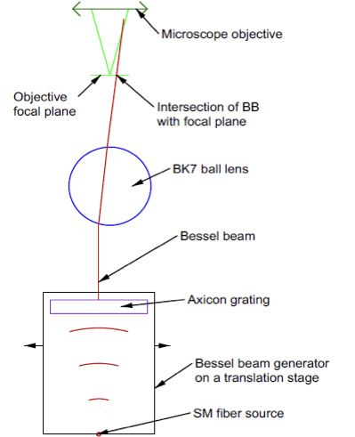
Fig. 1a. Schematic of the experimental setup

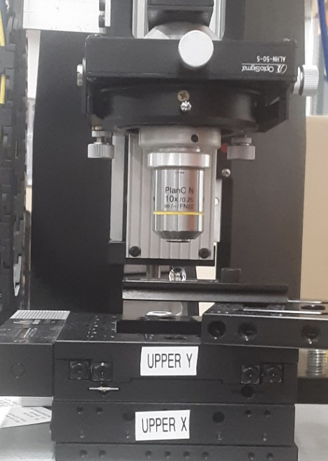
Fig. 1b. Setup showing ball in kinematic seat

As a vertical zero reference we use the Cat’s eye reflection from the upper pole of the ball and measure positive distances above the ball. For negative distances the objective is focused in the ball. The optical focal plane will be different from the physical focal plane because of refraction. Our measured vertical distances refer to the physical height of the focal plane.

Because the field of view of the 10x objective and camera are limited to about 1 mm we set an upper limit of the BB motion as ± 400 µm and viewed the BB as it moved through the field of view as in Fig. 2. We also wanted the experiment to simulate paraxial conditions as much as possible. 

The stage moved at a constant velocity from 400 to – 400 µm while the PSM software logged the spot position against a fixed time base. The slope of 2.795 means that the stage moved 2.795 µm per sample point. Notice there is a slight third order component to the spot position and a slight pause in motion toward the end of the travel. However, to a high degree the incident BB moves linearly with the stage motion. This means we can measure the spot position at the extremes of travel as being representative of measurement anywhere in the 400 to – 400 µm region.

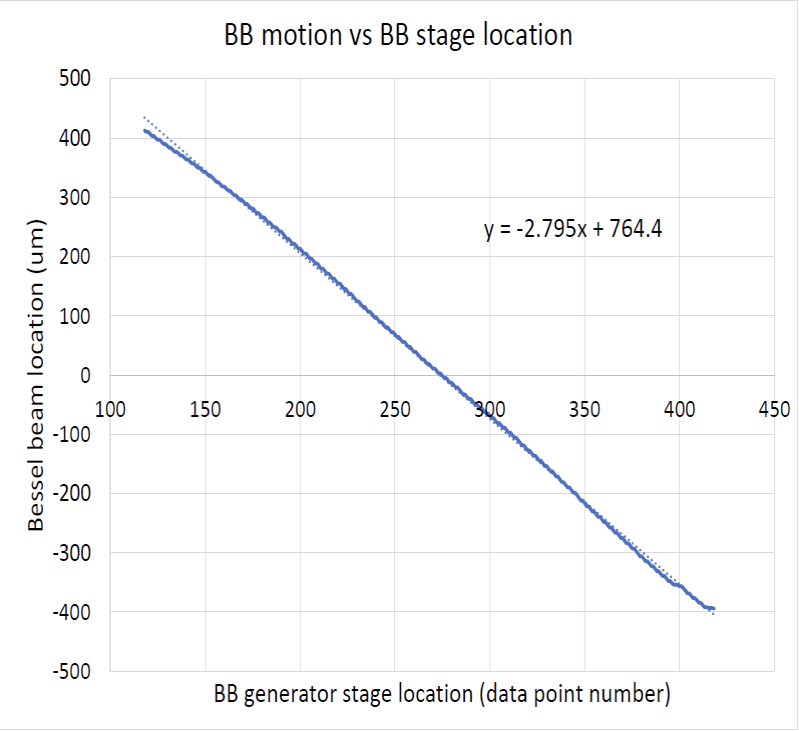
Fig. 2. Near linear BB position vs stage motion

Measurements of ray height were taken every 2 mm from 5 mm above the upper ball pole to – 5 mm below. These data are shown in Fig. 3. We took 3 measurements in the ball and 3 in free space to show the change in ray height was linear with axial height in both regions. We did not take a measurement at the back focus of the ball because the BB becomes an annulus at a focus and does not give a ray height.

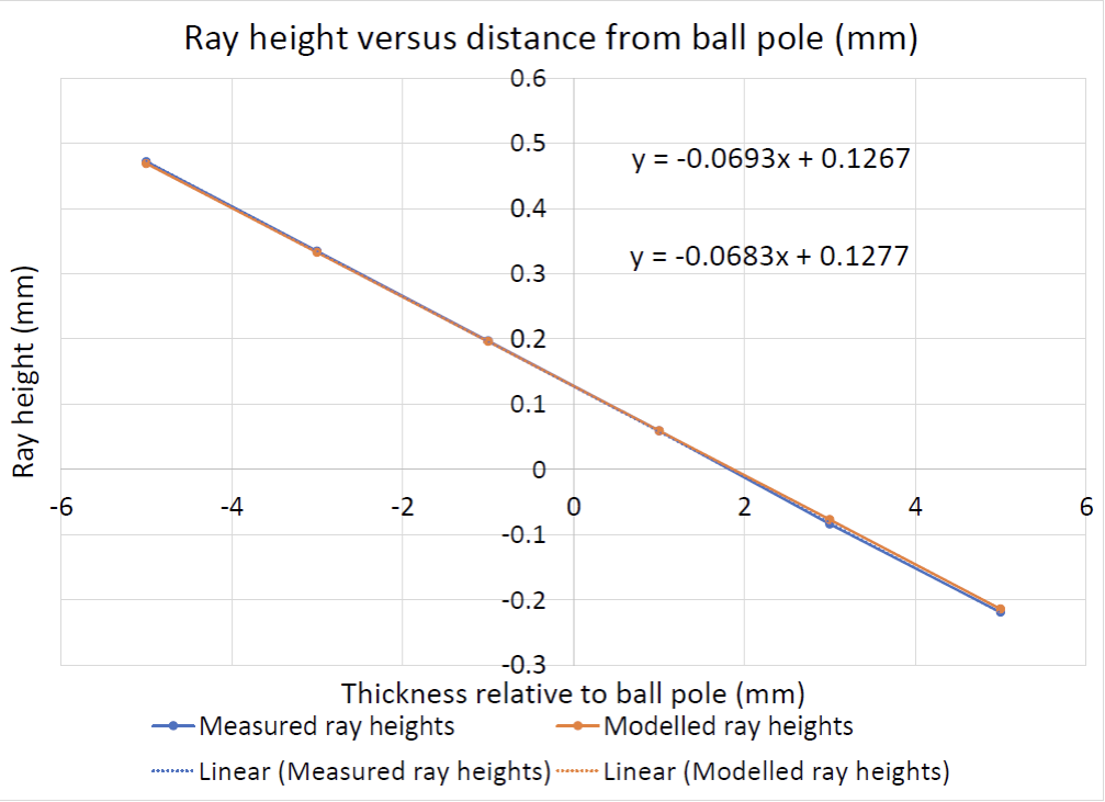
Fig. 3 Measured and modelled ray heights

Figure 3 is counter-intuitive in the sense that the negative half of the plot is of the ray height inside the ball and those heights are linear with those in free space as though there were no refraction at the glass air interface. Notice, too, that the ray height at 5 mm into the ball is about 0.47 mm, higher than where the ray entered the ball at 0.40 mm. Table 1 shows the measured versus modelled ray heights. 

Table 1. Measured and modelled ray heights

Height above pole (mm)	Measured ray height (mm)	Modelled ray height (mm)
5	-0.219	-0.214
3	-0.084	-0.077
1	0.059	0.059
-1	0.197	0.196
-3	0.335	0.333
-5	0.472	0.469

Notice the slope of – 0.0693 is close to the Zemax calculation of – 0.0683 of real ray heights versus distance from the ball pole for a ray incident from infinity at a height of 400 µm. 

To assure we were correctly taking the data, we would move the stage to ± 400 µm, record the ray height and then remove the ball to be sure the BB was incident on the ball based on the stage position. The position was correct and the error bars on the ray heights are on the order of ± 10 µm or less as seen in Table 1 and the orange curve of the modelled ray heights in Fig. 3.

LENS DESIGN MODEL

We used Zemax to model the ball lens. The model is shown in Table 2.

Table 2. Model values for the ball lens

Surface	Surface type	Radius	Thickness	Glass
Object	STANDARD	Infinity	Infinity
Dummy	STANDARD	Infinity	2
Lower pole	STANDARD	4	4	BK7
Ball center	STANDARD	Infinity	4	BK7
Upper pole	STANDARD	-4	5
Focal plane	STANDARD	Infinity

The final thickness of 5 mm means the microscope focal plane is 5 mm above the ball. To find the ray height at other distances, this value is changed. This model was used to calculate the model values in Table 1. The ray pathes at + and – 5 mm are shown in Fig. 4.

Fig. 4. Ray pathes from Zemax at – and + 5 mm

The ray pathes in Fig. 4 and the full pupil ray trace values in Table 3 help explain the reason it appears there is no refraction at the ball upper pole.

Table 3. Values from the full pupil ray trace

Comment	Y-coordinate	Z-coordinate	Y-tangent
Infinite object	Infinity	Infinity	0
Dummy	0.4000	-10.0000	0.0000
Ball bottom pole	0.4000	-7.9799	-0.0341
Ball physical center	0.2642	-4.0000	-0.0341
Ball top pole	0.1277	-0.0020	-0.0683
PSM focal plane	0.4693	-5.0000	-0.0683

Table 3 shows there is refraction at the top of the ball and that the slope of the exiting ray almost exactly doubles, not a coincidence but the fact the model is a ball lens. If the exiting ray is traced back into the ball as it is if we ask the ray height at – 5 mm, it starts at its height at the pole of .1277 mm  and continues at a slope of -.0683 for 5 mm to end up at a height of .4693, as in Table 3 and close to the meaured value in Table 1.

Finally, if we ask at what z height do the incident and refracted ray intersect we find (0.4-0.1267)/

-0.0693 = 0.2733/-0.0693 = -3.944 mm, very close to the pricipal plane of the ball lens.

CONCLUSIONS

We have shown in the case of a ball lens that a Bessel beam propagates through the lens as a single paraxial ray in a lens design program. The ball lens was chosen to illustrate this because it is impossible to introduce an error in the example due to tilt of the lens. 

While this is not a perfect experiment in the sense there is about a 1% descrepency between the predicted and measured ray heights, it is difficult to come to a conclusion other than the Bessel beam acting as a single paraxial ray. In doing any sort of experiment the precision of the results depends on the hardware available and the environment. The centroid of the BB can be located to ± 0.2 µm using a 10x objective, a 1 Mp camera and simple centroiding software. The main contributer the descrepency between experiment and theory is related to the stages that position the source, ball lens and microscope.

Clearly there is more work ahead in characterizing other examples of lenses and glass indices. While not reported explicitly in this paper, we have done experiments with a ball of a different index and at other axial distances. None of these results are inconsistant with the conclusion here.

In addition to reporting on other lens shapes including aspheres, and other indices, a theoretical verification of physical optics ray propagation is needed.

We end by a few words on the potential future impact of these results. For years lens systems have been designed based on multiple instances of tracing single rays but in the end the only method of accessing the alignment of the end product is based on the collection of all the rays filling the lens aperture. It was never possible to interrogate a single ray to see if it were going where it was predicted to go. 

By being able to define position and angle of a ray incident on an optical element or system and predicting where the ray will exit in position and angle, as we can from lens design or ABCD matrix algebra, we can locate the optical system in 5 degrees of freedom in space to a precision consistent with our knowlwdge of the ray positions and angles. In addition, the method may allow the wavefront measurement of aspheres and freeforms in a way that incorporates not only the manufacturing errors but the alignment.

ACKNOWLEDGMENTS

We would like to acknowledge the help of two J. C. Wyant College of Optical Sciences students, Karlene Karrfalt and Tyler Collins. One of us (REP) would like to acknowledge the help John Tesar, an independent optical consultant in Tucson, and  anonymous funding sources that have forced him to think harder about alignment.

REFERENCES

[1] Durnin, J. J. J. A. “Exact solutions fornondiffracting beams. I. The scalar theory.” JOSA A 4.4 (1987): 651-654.

[2]  Parks, Robert E. “Practical considerations forusing grating produced Bessel beams for alignment purposes.” Optomechanics and Optical Alignment. Vol. 11816. SPIE, 2021.

[3]    Nelson, W., et al. “Propagation of Bessel and Airy beams through atmospheric turbulence.” JOSA A 31.3 (2014): 603-609.

[4]  Turunen, Jari, Antti Vasara, and Ari T. Friberg. “Holographic generation of diffraction-free beams.” Applied optics 27.19 (1988): 3959-3962.

[5] Dong, Meimei, and Jixiong Pu. “On-axis irradiance distribution of axicons illuminated by spherical wave.” Optics & Laser Technology 39.6 (2007): 1258-1261.

[6] Santarsiero, M., “Propagation of generalized Bessel-Gauss beams through ABCD optical systems”, Opt. Commun. 132 (1996), 1.

[7] Parks, Robert E. “Rapid centering of optics.” Optifab 2021. Vol. 11889. SPIE, 2021.

[8] https://optiper.com/en/products/point-source-microscope