Author: csadmin

In Chapter 12, I commented again on classical optical instruments since there was interest in an earlier discussion. This got me thinking about what had changed in optical technology since the period ending about 1950 when there was a rather canonical set of classical optical metrology tools. There has been a huge technological change since then, yet little has been written about coherently integrating the changed pieces of technology. That is what I am going to try to do in this Chapter.

Virtually all optical systems have three major components: a light source, some optics that modify the light from the source, and a detector. I will address the changes in these three areas separately to give some order to the discussion and then summarize the consequences of the changes in designing new optical metrology instruments.

Light sources

In the years before the laser, that is, before 1960, man-made sources were either incandescent or some sort of electrical arc. Incandescent sources were physically large and not very bright but fairly stable in terms of position and intensity. Arc sources were brighter or could concentrate their brightness into a smaller size but were much harder to control in terms of the location of the brightness and its intensity level. Even when the HeNe laser came along and solved the brute intensity issue, workers went to great lengths to create point sources by using a microscope objective and a pinhole to “clean up” the source.

Today, I can create a bright, to-the-point-of-eye safety concerns, essentially perfect spherical wavefront with a single-mode optical fiber patch cord and a battery-operated 30 mW LED source used for testing optical fibers for continuity that sells for $20. (See, for example https://www.amazon.com/AKLTM-Visual-Fault-Locator-Tester) The only practical downside to this source is that it is too bright for some applications, and the intensity is not adjustable. There are commercially available laser diode sources that are perfect for illuminating a single-mode fiber, are fully adjustable from pW to mW, and are available in various wavelengths from NUV to NIR. These low-power, adjustable sources typically cost 50-100x the battery-operated ones, but you have control and stability.

Optical elements

Between the source and detector are optics that modify the light before it reaches the detector. Various optical elements could go here, but I will stick to lenses and mirrors. About the time of the invention of the laser, you could begin to buy lenses out of a catalog, with Edmund Optics leading the way. This made it much easier for someone to try out a particular combination of lenses on an optical bench to prototype a new system without waiting for custom (and expensive) optics to experiment with.

Another development starting about the same time was computer-aided lens design. This meant there was more variety in optical systems that could be assembled without much expense and delay because designing new optical systems was easier. This development led to a commercial market for impressive photographic camera lenses. At the same time, governments realized it was much easier to spy on everyone with sophisticated telescopes in planes and satellites.

This, in turn, led to testing optics interferometrically to make better-quality optics than previously. Once testing was easy, there was a push toward deterministic polishing methods, such as the MRF technique developed by QED Technologies. This meant that the lenses listed in catalogs were sufficiently high quality that diffraction-limited systems could be laid out on a tabletop optical bench. The only obstacle to diffraction-limited performance was the precision of the optics’ alignment.

Detectors

Before about 1970, most images were captured on photographic film, a reliable and inexpensive method of capturing and storing massive amounts of data. However, if your camera loaded with film was in space and you wanted to see the pictures, there was a problem. The other demand came from photographers with expensive lenses who wanted to see the results of their pictures sooner rather than later. This led to the development of electronic cameras, but because they used the newest technology, they were pricey. If you had a spy satellite or a large terrestrial telescope, you could afford an electronic camera, but they were not affordable for the general public before about 2000.

For scientific use, electronic cameras are incredibly useful. An easily affordable megapixel camera with a shutter speed range of microseconds to seconds and additional gain was readily available by 2005. Such a camera coupled with microscope optics was capable of diffraction-limited imaging with a 10 x objective over a 1 mm square field of view with instant image availability for further processing. One could argue that photographic film has a higher data storage density than an electronic camera. However, in conjunction with its associated computer, the electronic camera is so much more flexible as a data interface that it is the obvious choice for data capture.

The whole is greater than the sum of the parts

When you consider an autocollimating or autostigmatic optical instrument that incorporates a light source, optics to project and receive light from the source, and a camera to capture and store the image, you now have much more to work with than they did in the day of the classic instruments. Between the adjustability of the light source and the camera you have a useful range of intensity variation of something on the order of 1010. The data cube in one megapixel, 16-bit image is in the same order.

During initial alignment to get reflected light into the instrument, you can turn the laser to its maximum 1 mW level for a Class 1 laser device and see the light under many ambient lab lighting conditions, so you don’t have to darken the lab to find the light. Once the light is back in your instrument, you don’t have to work your head into an odd angle to view in an eyepiece; you can comfortably observe the image on a monitor. Finding a zero setting or finding coincidence is no longer subjective; you get a repeatable, objective number on a monitor. You don’t have to write down your measurement result; you tap a key to store the result or the whole image on a computer that controls the instrument.

Implication of technological changes on the mechanical design of classic optical instruments.

If you knew nothing about the design considerations of classical optical metrology instruments, think of autocollimators as an example, but had today’s technological resources, would you design an autocollimator to look like a classic example? I argue, no. Would the new instrument have a large aperture? No. You get plenty of light back into a small aperture with a laser source.

Would you use a round, precision-ground barrel as a mechanical datum to aid in setting the crosshair to the center of the aperture? No, you can set zero by pointing the instrument at a small retroreflector. Would you use an incandescent light source that draws 10 or more Watts or a laser diode that draws 10 mW? Would you use the new technology for light sources and cameras but then attach it to a custom controller for readout? No, you would attach your device to a generic computer via a USB cable and put the custom controller and readout into the software on the computer.

I conclude that with the new technology, classical optical instruments can retain their same function and accuracy without requiring the older instruments’ mass, size, external features, and electrical demands. No, the new instruments will not look the same as the old or be massive, yet they will perform the same function as well or better than the old. The hurdle is to set aside the picture of a classic autocollimator and ask where is the modern functional equivalent. Optical metrology instruments using the new technology are now catalog or online store items.

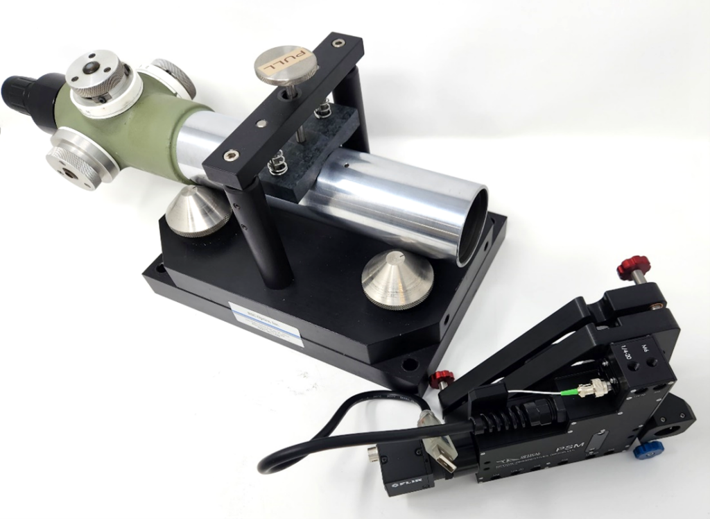
The old and the new with greater functionality using today’s technology

There was more interest in Chapter 3 about the classical instruments used for optical alignment than any other chapter to date, and I didn’t have a chance to say all I wanted to, so I will continue the discussion in this Chapter to emphasize how changes in technology have changed the design of these instruments. The instruments discussed previously are basically the same; they increase the angular sensitivity of the eye from about 1 minute of arc to something substantially greater by using two lenses of different focal lengths to increase the magnification of the eye.

The objective and eyepiece in a telescope change the angular extent of a distant object into an image that subtends a much larger angle as the nearly collimated light enters the eye from the eyepiece. A microscope is nothing more than a telescope with a short focal length lens out in front to make small objects look larger by the ratio of the microscope objective to the telescope objective’s focal lengths. In this case, the telescope objective is known as the tube lens in microscope speak.

In the 17th century, when the telescope and the microscope were invented, the only illumination source was natural light. The object was directly illuminated in the case of the telescope, or natural light was reflected on the object by an auxiliary plane mirror for the microscope. Starting around 1830, candles and other types of lamps were used with microscopes for illumination [1].  This type of illumination would be impossible to use with any optical alignment instrument because these are double-pass instruments that project a reticle pattern, such as a crosshair, and view it in reflection. 

The use of a crosshair or reticle pattern started in the 17th century, and Robert Hooke is given credit for the invention [2]. A crosshair is easy to install in a single-pass telescope or microscope, such as an astronomical or transit telescope for surveying. For double-pass optical instruments, illuminating a crosshair for projection was impractical before incandescent bulbs became available. These were not even available in small enough sizes to install inside the instrument around the early 1900s. The Drysdale paper from 1900 describing the autostigmatic microscope in Chapter 3 is vague on the illumination source, a probable indication of using natural light.

Even with a useful-sized bulb, the bulb illuminated a frosted window inscribed with the crosshair, reducing the light available for viewing the crosshair. A clear window would make the bulb filament visible and make a distracting background. The relatively low level of illumination of the crosshair is what makes finding the return reflection from an autocollimator so difficult. This is why lab lights are dimmed, and a flashlight is pointed down the eyepiece on an autocollimator to aid in finding the return reflection, and in this case, the alignment is just in two degrees of freedom.

[Sidebar] Before going further about the design of classical optical alignment instruments, let me mention a classic publication about them: Optical Instruments and their Applications, By Douglas F. Horne, published in 1980 by Adam Hilger, Ltd. The book goes into detail with chapters about telescopes, microscopes, cameras for commercial and industrial purposes, surveying instruments, aerial photography and photogrammetry. The chapter on Engineering Metrology covers the instruments I reviewed in chapter 3, alignment telescopes and autocollimators, and the tooling used with them, such as right angle squares and angle gauge blocks, but curiously omits autostigmatic microscopes. Many pictures of the optical paths in these instruments show how the reticles are illuminated. Unfortunately, the book is out of print but may be available in some libraries.

Once the laser was invented in 1960, the lack of a bright light source was solved. Further, coupling a laser to a single-mode fiber produces a near-perfect spherical wavefront. When this spherical wavefront is collimated, a plane wavefront is created that is useful for autocollimators. This wavefront is reimaged as a several micrometer diameter spot on the detector in the autocollimator, leading to sub-microradian angular sensitivity when coupled with a sufficiently long focal length collimating lens. A 100 mm focal length autocollimator has a 1-2 µradian sensitivity using a CMOS camera as a detector.

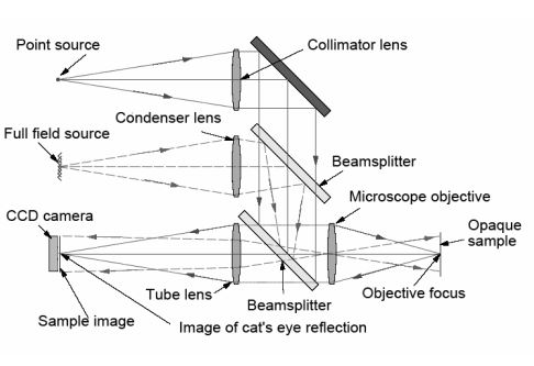
In addition to the laser/fiber combination increasing the resolution, the higher brightness makes the initial alignment of the mirror to the autocollimator easier because the reflected beam is more easily seen under ambient lighting conditions. This angular alignment only concerns two degrees of freedom. To align an autostigmatic microscope that can be thought of as an autocollimator with a microscope objective added on the front, see Figure below, three degrees of translational freedom are involved. This requires even more light to find the location of the reflected spot and get the spot in the small volume of space that the detector can see.

It may seem counterintuitive, but the axial degree of freedom is the most difficult to locate. This is because the focused cone of light spreads out, and its intensity varies as the square of the distance from focus. One must be in the correct axial position to a mm or so to see the focused spot using a 1 mW laser under ambient lighting.

As with the autocollimator, as soon as just a bit of the reflected light enters the microscope objective, the alignment is easy to finish. In fact, with modern digital detectors, the 1 mW source is orders of magnitude too bright to avoid saturated pixels when the reimaged spot is in focus.

In a carryover from past instrument designs, most current autocollimators and centering equipment display an electronic crosshair that simulates what you would see looking into the eyepiece of an older instrument. I prefer to look at the reflected spot image itself because the spot contains information lost with the simulated crosshair. As little as a 10th wave error in the surface being viewed will distort the reflected, nominally perfectly circular spot. Because of this, it is immediately obvious if something is wrong with the object being viewed.

I remember long ago viewing a 300 mm diameter spherical mirror at its center of curvature. The technician behind the mirror adjusting the mount to align the center of curvature to my autostigmatic microscope was surprised when I told him the mirror was too tightly clamped. He said, “That can’t be; it’s only finger tight.” I had him look at the image of three distinct flares at 120° apart. He shrugged his shoulders and said, “Oh,” and went back and loosened the mounting screws.

More recently, much the same thing happened in a government lab using a point source microscope (PSM). The user thought something was wrong with his PSM and had sent me a picture of the image. I suggested he check the mount, and he found that it was the mount, not the PSM, that was at fault. These are examples of situations where if the problem is misunderstood, the error can creep into work farther down the line, where it is even harder to figure out what went wrong. It is much better to find out early, which is easy to do if viewing the real image rather than a simulated crosshair.

[Sidebar] A good reference for looking at images (and that is in print) is Star Testing Astronomical Telescopes by H. R. Suiter, published by Willman-Bell, Inc. (1997). The book has many photographs of star images through focus and of misaligned, poorly mounted and roughly polished surfaces. This gives you a good idea of the kind of images you can see in an autostigmatic microscope that uses a single-mode fiber as a “star.”

There is an additional benefit to directly viewing the reflected image. The same sort of software that aids in aligning astronomical telescopes can be used with a fiber or pinhole-illuminated autostigmatic microscope to give quantitative wavefront information. Here I refer you to
https://www.innovationsforesight.com/product-category/software/skywave/

To recap, the optical principles of modern optical instruments are no different from those used 200-300 years ago. What is different are the sources of illumination, orders of magnitude more intense (the laser or LEDs), and more spatially controlled via optical fibers, computer-generated patterns, and spatial light modulators. On the receiving end, digital cameras are many times more sensitive than the eye. Because of a large range of shutter control, they work well over orders of magnitude of incident intensity. Combining a high-brightness source and the ability to control that intensity at the detector gives modern optical alignment instruments a sensitivity and flexibility that is impossible using the eye as the detector.

In future chapters, we will cover additional flexibility provided by the analysis of structured illumination to provide a third dimension of information from nominally two-dimensional intensity distributions.

[1] Davidson, B. M., “Sources of illumination for the Microscope 1650-1950”, Microscopy, 36, pp. 369-86, (Jan-June 1990)

[2]https://en.wikipedia.org/wiki/Reticle#:~:text=Most%20commonly%20associated%20with%20telescop ic,dates%20to%20the%2017th%20century.

As I said in the first chapter, I hope to make these articles into a book on alignment after significant editing to organize the material coherently. In that spirit, and before I forget, let me discuss some aspects of alignment and precision engineering that belong in a Preface or Introduction to the book rather than here. My motivation is returning from a meeting of the American Society for Precision Engineering, where I took a tutorial on alignment from Vivek Badami of Zygo and Eric Buice from Lawrence Berkeley National Laboratory. You might ask why since I am writing on this subject, but everyone views alignment from a different perspective, and there are aspects of the subject that you might never have thought of but are essential to others. For example, Eric is interested in the alignment of magnets in an accelerator using a wire as the detector of the axis of the magnetic field.

From the alignment tutorial and papers at the meeting, a couple of principles of precision engineering stand out. How well you can make measurements depends on the environment you are working in. At least three significant causes of disturbance exist: thermal effects, vibration, and air turbulence. To give concrete examples, I have attached a paper written several years ago about a large machine tool that illustrates these effects nicely. For each category, I refer to the illustration in the paper. For the details, please see the paper itself.

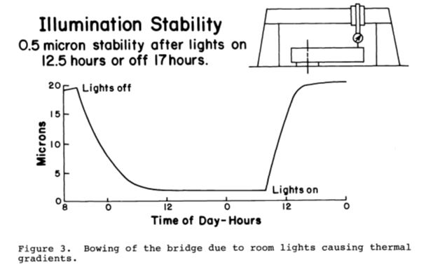
Thermal effects cause dimensional changes in most materials, and at the µm level and below, people worry about temperature changes of millidegrees. These dimensional changes cause drift and a lack of repeatability. The first example in the paper deals with the lights in the room where the machine was installed. Being conservation-minded folks, we turned the light off in the evening and back on when we got to work in the morning. Unfortunately, this caused an 18 µm change between the tool and workpiece and took most of the workday to stabilize. We just left the lights on all the time, as in Figure 3.

Figure 4 in the paper shows that 0.1° F. change in room temperature will cause a damped reduced temperature of the steel in the machine. The nominal control of the room temperature to 0.02° for several hours was enough to make this a minor contributor to machine errors.

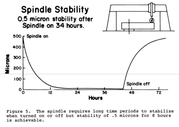
The biggest thermal effect was running the machine spindle. It elongated by 0.5 mm over a 20-hour period. Again, leaving the spindle running except for changing wheels was the only solution, as in Fig 5. In general, thermal effects are categorized as systematic effects; they are relatively long-term effects compared to the time needed to correct for the effect by some feedback mechanism.

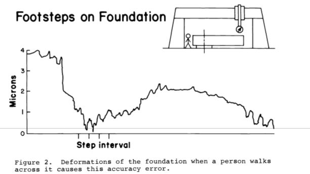
In the vibration category, we usually think of seismic vibration coming up through the floor and forget about acoustic vibration. However, even when taking precautions, as shown in Fig. 2, it pays to stay off isolated foundations and avoid touching isolated optical tables during experiments. Leave your laptop off the table and as far away from the experiment as possible. It is a source of vibration and thermal effects.

Acoustic vibrations also have consequences. While I can’t document this, I remember watching a part being diamond-turned at Oak Ridge National Laboratory. They had a claxon to signal for an incoming phone call.  You could see the change in the part’s surface finish from several feet away when the claxon sounded. In another case, having flooring too near the underside of an isolated optical table is a problem. Walking on the floor transfers deflections in the floor to the table because the air between couples the flooring to the table. Here I speak from experience. Opening the gap a couple of inches fixed the problem. The effect of both kinds of vibration combines systematic and statistical noise. Sometimes isolating your experiment from the environment is easy, but just when you think you have it isolated, another source of vibration pops up.

Anyone who has used an interferometer is aware of air turbulence. The irregular change in the shape of the fringes is a sure sign of turbulence. It is also visible in the image using an autostigmatic microscope (ASM). The image’s centroid will dance around, and the flair around the edges of a well-focused spot will change. This type of noise is largely statistical, and the practical method of reducing statistical noise is through averaging. One area of precision engineering that has made large steps here is the astronomical community, which combines wavefront sensing and deformable correction optics to improve the images of stars and galaxies dramatically.

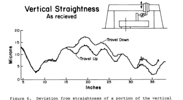
This thought brings me to another impediment to precision, at the µm level, everything is deformable, and to first order, all materials should be considered rubber. Fig. 6 in the paper is a beautiful example.

The ways along which the tool spindle moved were ground steel blocks with a cross-section of 50 by 150 mm. As the spindle moved past the bolts that held the ways together, there was a roughly 10 µm bulge every 150 mm due to over-tightened bolts. Loosening the bolts largely corrected this straightness error. Since the stiffness of plates varies as the thickness cubed, it is easy to see why the least stress will distort thin plates such as lenses and mirrors.

This is probably enough on the difficulty of doing precision work, but it leads to a topic I want to discuss in the next chapter, once you have aligned a system, how do you secure the alignment? The tutorial I attended had a good discussion of this topic, and I will share some of their thoughts in the next installment.