Chapter 5: Optical Axis Definition

The purpose of optical alignment is making the optical axis of an optical element, or complete system, coaxial with some other axis that is defined by other optical or mechanical components. This means we must start the discussion of optical alignment by making sure we all mean the same thing when we say the optical axis of a lens.

For a singlet optical element, the definition is simple. The optical axis is the line joining the centers of curvature of the two surfaces. The green arrows in Fig. 1 start at the physical centers of curvature. The red solid arrows start on the optical axis at the optical centers of curvature, that is, the position along the optical axis where the center of curvature appears located due to refraction at the intervening surface when viewed with an autostigmatic microscope (ASM) or an alignment telescope (AT). We will look at the process of using either of these instruments in a subsequent chapter. For now, we are just dealing with the definition.

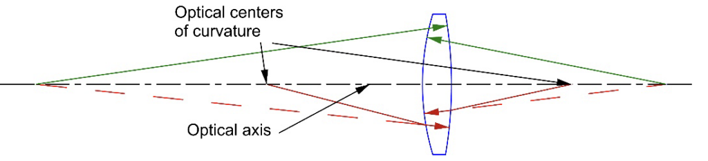
Fig. 1 Physical and optical centers of curvature that define the optical axis of a single lens

We know one way of defining a line is with two points and those two points are uniquely defined here by the two centers of curvature as in Fig. 1. Independent of whether the surfaces are concave or convex, the optical axis is always normal at its intersection with the surfaces because the axis passes through the centers of curvature. This means here is no refraction or deviation of a ray propagating along the optical axis in either position or angle. This fact is implicit in the definition but seldom stated.

The definition shows why the optical axis is so important to alignment. When a lens is aligned to a reference axis and there is no deviation of a ray propagating along the reference axis the lens is perfectly aligned to the reference axis in tilt and decenter.

(Sidebar – There is a trap in this definition if you don’t think it all the way through. Say I have a lens and I want to center it in a collimated beam relative to some fiducial or datum perpendicular to the beam. I align my ASM or AT to the datum and insert the lens.  By tilting and decentering the lens I get the back focus well centered in my instrument. The image is well centered but by eye the lens looks tilted.

The trap is that I have tried to center the lens using the back focus only. That is a single point, so I only know 3 degrees of freedom (DOF) and I am trying to determine an axis, or a line. I need 4 DOF to do that. I do not have enough information to know the lens is centered, that is, whether the optical axis of the lens is parallel to the axis of the collimated beam. I need a second point such as the center of curvature of one of the surfaces to know the lens is completely centered.)

Optical axis of multiple elements

In looking for a definition of the optical axis of a real assembly of optical elements rather than the design of an assembly I stumbled upon this note by A. E. Conrady [1] from 1919 that states the situation I am discussing perfectly.

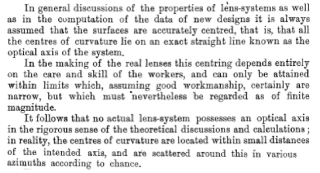
So, what is the “optical axis” of set of centers of curvature “scattered around…according to chance”? For the purposes of our discussion, I propose it is the analogue of the optical axis for a single element in a functional sense. What does the “scatter” do to the deviation of a ray propagating through the assembly? My definition is when the optical axis of an assembly of lenses is aligned to a reference axis an optical ray co-axial with the reference axis is not deviated in position or angle while passing through the lens. This begs the question of how we create a single optical ray, but we will get into that in another couple of Chapters.

The same trap occurs here as for the single element. When the system is aligned to the reference axis we must probe the transmitted ray at two distances from the lens to assure that neither the angle of the ray nor its position has changed. This aspect of the problem is getting ahead of myself, but I think you will agree that the definition makes sense assuming we can measure the transmitted ray.

Example of the optical axis definition for a “system” of elements

Consider a cemented doublet whose prescription is shown in Table 1. If the doublet is perfectly centered, the centers of curvature of all three surfaces lie on a straight line that is both the mechanical and optical axis as in Fig. 2a. If there is an error in cementing this is no longer the case. Assume there is a 30 minute of the meniscus relative to the positive element. This is about 10 times larger than the typical centering tolerance for an off the shelf doublet but the large decenter makes it possible to see the errors in Fig. 2

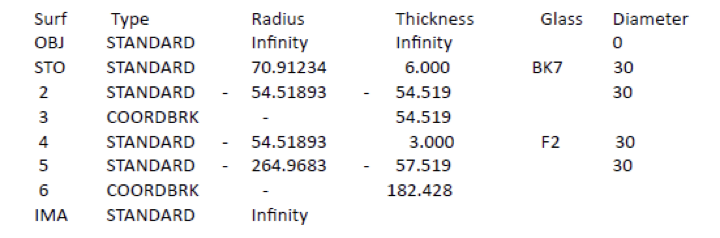
Table 1 Prescription of the cemented doublet used in the example

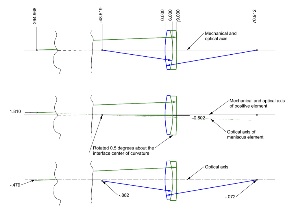
When the meniscus is rotated about the center of curvature of the 2^nd surface of the positive element, the center of curvature of the 2^nd surface of the meniscus moves 1.81 mm above the optical axis of the positive element. The mechanical vertex of the meniscus is about half a mm below the axis as seen in Fig. 2 (middle) 

To find the optical axis of this “system” the doublet is allowed to rotate and decenter about the 1^st surface of the positive element relative to the initial optical axis of the perfectly centered doublet until the transmitted ray traveling along the initial axis in neither changed in position (ray height) or angle. A ray trace optimization program calculates the doublet must be rotated 0.389° CCW and decentered downward 0.553 mm for no deviation of the ray.

The correction places the centers of curvature of all 3 surfaces below the optical axis as in the lower part of Fig. 2. The centroid of the image formed at the back focus of the lens for a collimated beam parallel to the original axis would shift about 0.01 mm from the optical axis. Because a tilt about 10 times a typical tilt was used in the example, we get an idea of what to expect from a typical lens by scaling back a factor of 10. A 3 minute tilt is barely perceptible in most instances.

Throughout this discussion we have talked about using a single ray to establish the optical axis. Creating this single reference ray is discussed in a future Chapter.

Other definitions relating to alignment

Before talking about how to use optical instruments to align optics it is helpful to define a few more concepts. We will finish out this segment with these thoughts.

First, we have pointed out that a line, or axis, is defined by 2 points, or a point and 2 angles, 4 DOF altogether. Do not forget that a circle of any radius can be drawn through 2 points. To show 2 points lie on a straight line you need to measure a 3^rd point and prove it lies on the same line.

Next, a plane mirror is a plane defined by 3 points, or 3 DOF. This is why you need 2 plane mirrors to turn an axis from one position and angle to another position and angle. There are not enough DOF to do it with one plane mirror. You need 4 DOF to define an axis. A good example are orthogonal galvo scan mirrors. You need 2 mirrors to scan over all angles in a hemisphere where the beam starts from a particular location and angle.

A spherical mirror or surface is defined by 3 DOF to determine the location of its center of curvature. You need a 4^th point to know its radius of curvature. This is why when using a coordinate measuring machine (CMM), you need to touch the master ball in at least 4 places for the machine to know where the center of the ball is. This is the perfect example of a difference between optical and mechanical measurements, and why we can say that a spherical ball, or any part of a spherical surface, is an analog of a point. If a point source of light is at the center of a spherical surface the light will be perfectly reflected back on itself to the point independent of the radius of the spherical surface. 

For a mechanical measurement we need to also know the radius of the surface to know when the center of curvature is located. Not only do we need 4 points, but in the case of a concave mirror, 4 points around the edge won’t do. We need one point near the middle of the mirror to avoid an ill-conditioned situation that makes the calculation of the center of curvature a poor estimate. Further, most people do not like you to touch the middle of an optical surface. The safest method of finding the center of curvature of an optical surface is to do it optically. This is also the quickest and most precise method of finding the center of curvature.

This is why when using a coordinate measuring machine (CMM), you need to touch the master ball in at least 4 places for the machine to know where the center of the ball is. 

Cylinder – The next most complex surface is a cylinder that is defined by its axis, or 4 DOF. As an analog to a spherical surface, you can find the axis of a cylinder of any radius with 4 DOF, but you need a 5^th point to determine the radius of curvature of the cylinder, just as you needed 3 DOF to find the center of curvature optically but a 4^th point to find the radius. When a point source of light is focused at one of the axes of a cylinder the reflected light comes back to form a line image. Using an autostigmatic microscope you can find the axis in 3 DOF, 2 DOF in translation and 1 in angle.

Symmetric asphere – A symmetric asphere also requires (for alignment purposes) 4 DOF to define because as opposed to a spherical surface, a symmetrical asphere has an axis. A 5^th point is required to define its vertex radius of curvature. We will get into more details about aspheres later but for now these are the basic alignment details.

Off-axis asphere and a toroid – An off-axis asphere requires 5 DOF with an addition point to define a radius in one direction. Toroids are included here because if you mask or stop down an off-axis asphere you effectively are left with a surface with 2 cylindrical surfaces of different radii at right angles to each other. There are cases where a toroid will be a satisfactory substitute for an off axis asphere just as a sphere can substitute for a symmetric asphere if the f/# of the surface is slow enough.

This is enough on definitions. In the next Chapter we will get into the first steps of classical alignment.

[1] Conrady, A. E. (1919). Lens-systems, decentered. Monthly Notices of the Royal Astronomical Society, Vol. 79, p. 384-390, 79, 384-390.