This webinar with Robert Parks is presented by the OSA Systems and Instrumentation Technical Group.
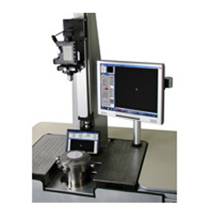
Topics discussed include the evolution of the classical autostigmatic microscope (ASM) into an all-purpose optical alignment tool whose use has been described in over 60 optical engineering papers that illustrate real-world systems applications.
The evolution that led to the current instrument, the Point Source Microscope or PSM, is due to a convergence in technologies of solid state light sources, digital cameras, modest cost computers and software to operate these devices to create a small, lightweight and ergonomic optical test instrument with many functions.
WHAT YOU WILL LEARN IN THE WEBINAR:
Viewers will learn the fundamentals of autostigmatic microscopes and how they are used to find the radius of curvature of optical surfaces. This background into fundamentals leads to discussing the use of the ASM in practical alignment situations.
Viewers will be presented with a variety of applications of the ASM to the alignment of optical systems, particularly applications that include aspheres and folded optics to give an appreciation for the capabilities of this technology.
MFT was mentioned in five of the papers given at the SPIE Conference on Telescopes in Edinburgh, Scotland at the end of June 2016 by authors from six different international research organizations.
PROC. SPIE 99055O, SEE MENTION OF MFT ON P. 19, FIG 18.
The surface roughness measurements of a silicon plate with a multilayer coating to reflect Xrays taken with the MFT are consistent with each other going from 2.5x to 10x magnification, consistent with the atomic force microscope for higher spatial frequency measurements and consistent with the model of the surface roughness. The figure shows a map of the surface taken with the MFT, upper left, and a graph showing the consistency of the various measurements and the model over many orders of magnitude of spatial scale.
PROC. SPIE 99120O, MFT NOTED ON P. 10, FIGS. 16 & 17
Shows the MFT sitting on the 4.2 m mirror and the lap top computer sitting along side it with a map of the mirror surface on the screen. Figure 17 shows 3 examples of the surface roughness taken at 3 different places on the mirror but all giving results in the 1 nm rms range over a sample area of 3 x 2.4 mm. Figure 18 shows that these surface roughness measurements converted into BRDF illustrate the mirror finish meeting the specification. It had previously been shown that the bare Zerodur mirror could not have been measured directly for BRDF because of the polycrystalline nature of the substrate but by measuring the surface roughness there was a path to measuring and meeting the specification (see Tayabaly, et. al., “Use of the surface PSD and incident angle adjustments to investigate near specular scatter from smooth surfaces”, Proc. SPIE 883805, 2013).
PROC. SPIE 960307, MFT MENTIONED ON P. 6 AND FIG. 2
Roughness tolerances for Cherenkov telescope mirrors on p. 5-6 and Fig 2, gives a description of the MFT in detail and shows the MFT sitting on a Cherenkov mirror substrate and an example of the surface roughness of the dielectrically coated mirror that was about 1 nm rms. The paper goes on to show that a variety of mirror substrates and coatings were measured for surface roughness and the resulting surface roughness maps are shown in Fig. 3 that range from 0.58 nm rms to about 12 nm rms depending on coating and exposure to the environment.
PROC. SPIE 99120Q, RESULTS OF MFT MEASUREMENT ON P. 6 AND FIG. 9
Polishing and testing of the 3.4 m diameter f/1.5 primary mirror of the INO telescope, p. 7, Fig 9 shows the results of 156 separate measurements made on various parts of the mirror with an average roughness of 0.6 nm rms. This was a mirror made of Zerodur so the surface roughness could not be measured using scattering, and surface roughness had to be used to see that the mirror met spec. Also, because of the speed of the mirror it would have been difficult and time consuming to have made replicas to measure the surface roughness.
PROC.SPIE 990578, MFT RESULTS ON PP. 4-5 AND FIGS. 5 & 6
Ion beam figuring of thin glass plates: achievements and perspectives, P 4-5 and Figs. 5-6, indicates the MFT was used to measure the surface roughness of ion beam polished glass plates only 0.4 mm thick, yet because of the low mass of the MFT it was possible to set the MFT directly on the thin plates to make the measurements. Figs. 5 and 6 show the surface roughness maps after various amounts of material was removed by ion beam polishing and the resulting change in roughness. The places on the substrates were carefully aligned so that it was possible to show the evolution of the change in roughness. Again the data were highly consistent. Special mention was made of the low mass being particularly useful in this study.
The main reason is that the other two major factors in performance, optical design and optical fabrication, have already been improved to the very limits of what can be accomplished. After spending good money on a near perfect design and fabrication of optical components does it make any sense not to assemble them in perfect alignment?
By perfect alignment we mean placing the elements where the design says they should in the theoretical optical and mechanical design, not just within some tolerance band, but precisely where the design says they should be. Only this way can you get performance at the same level as the perfection of the design and fabrication of the components.
In the last several decades with the help of incredible computing power optical design has reached the limits of perfection. Optical systems are being designed with vastly better performance than ever before by making use of aspheres and coatings that could only be used because of the computing power available these days. Unfortunately these advanced designs could not be made because optical fabrication methods had not kept up with the power of optical design.
Now with computer controlled polishing techniques like MRF, diamond turning and molding of both glass and plastic elements the aspheres that help with performance because of their design are now practical to make to high quality. Similarly coatings to enhance performance have been improved to the point that making them any better is no longer cost effective.
Now comes the hard part; how do you position these near perfect components, mechanical and optical, relative to each other so they perform as well as the theoretically perfect design? One way, the way usually followed is to tighten the tolerances on both the optical and mechanical parts until they have to go together perfectly but this is impossible to do because some slop has to be left or it is impossible to get the glass into the metal mount.
Another way is to leave loose tolerances for edging and bores of lens barrels so the element can be positioned where the design specifies it should be. This is where a tool like the PSM comes in. The PSM can be positioned so its focus is where the center of curvature of a surface should be according to the design and then the surface adjusted until it is centered to the PSM reference cross hairs.
Clearly this is not the way to assemble optics on a mass production basis. But when performance is at a premium such as in lenses for reconnaissance and cinematography, for example, it is far more efficient and cost effective to allow looser tolerances on glass and metal, and then individually align each element as it should be.
I remember many years ago seeing sophisticated lens systems assembled from well-made glass and metal components which were then tested for optical performance. They often failed the optical test and were sent back to the assembly department where they were taken completely apart and re-assembled with the hope that this time they might pass the performance test. In hindsight this was a ridiculous procedure. With the aid a a PSM and a little Fixturing the lens systems could have been assembled so they passed the optical test the first time, every time. This is the smart way to do alignment.
Measuring the radius of curvature of a concave surface – Main historical use
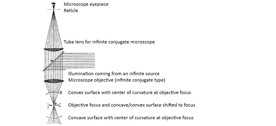
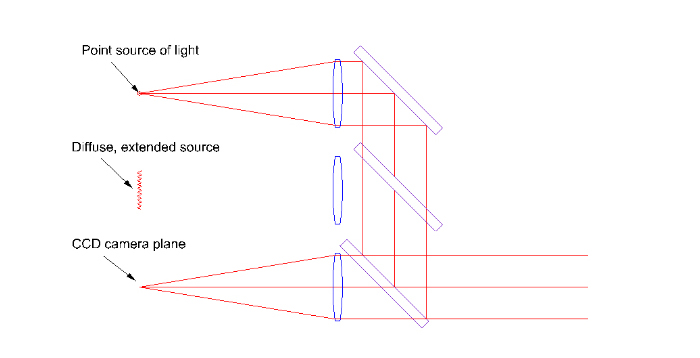
Modern version of an ASM uses internal infinite conjugate optics
Use of an ASM for alignment of optical systems
Other uses of an ASM
Conclusions
DESCRIPTION OF AN ASM
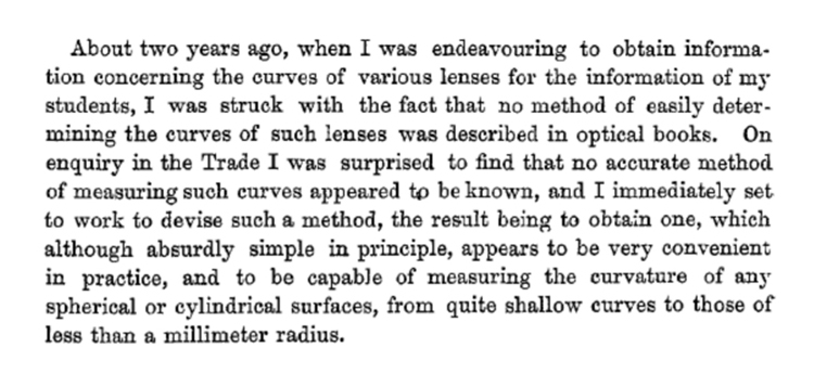
First description in English literature is Drysdale, Trans. Opt. Soc. London, 1900
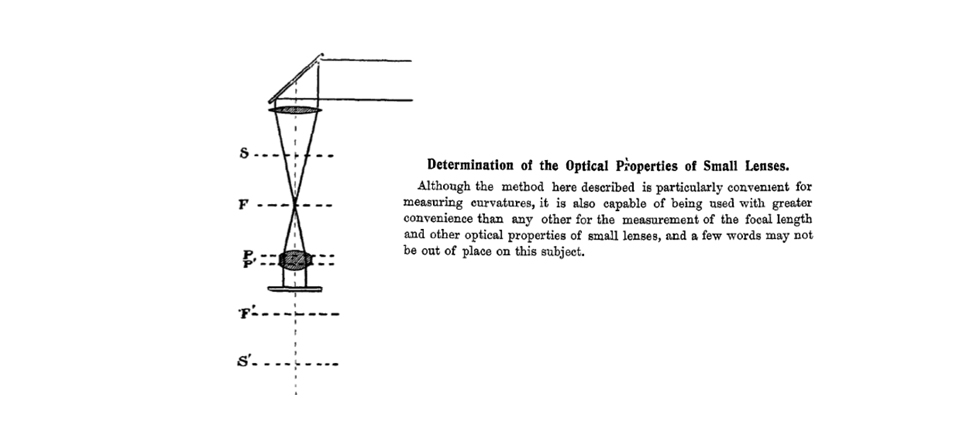
Fig. 2 from the Drysdale paper of 1900
Further from the Drysdale paper
CAT’S EYE AND CONFOCAL FOCI
CAT’S EYE
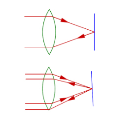
Cat’s eye reflection
Objective focused on surface
Out going rays re-enter on opposite side of objective
If surface tilted, reflected rays parallel outgoing rays in collimated space
Cat’s eye used for setting crosshairs
Cat’s eye used for setting reference
CONFOCAL FOCI
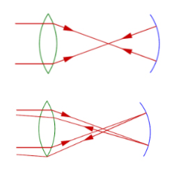
Confocal reflection
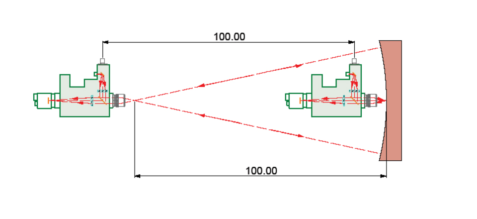
Rays focused at center of curvature
Rays hit surface at near normal incidence and re-trace themselves
If surface tilted, rays do not re-trace and will not center on crosshairs
Confocal used for alignment
Confocal for bringing CofC to reference
EXAMPLES OF CAT’S EYE AND COFC SPOT IMAGES
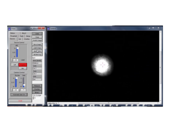
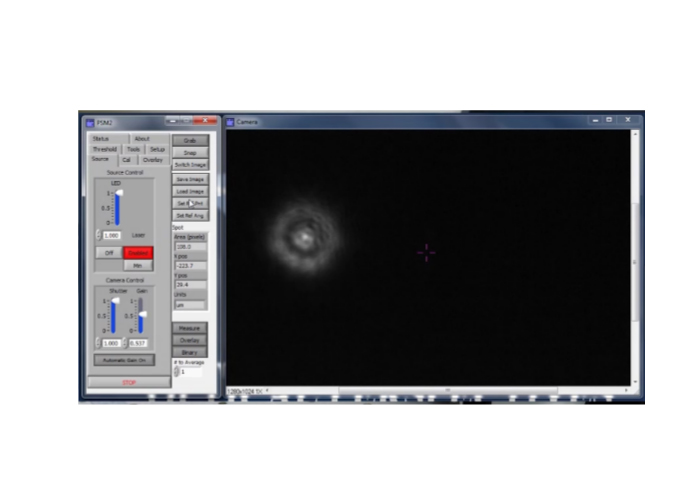
OUT OF FOCUS CAT’S EYE SPOT IMAGE
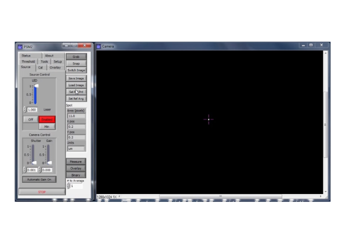
IN FOCUS CAT’S EYE
Notice Shutter and Gain with focus
Locating an ephemeral point in space with 3 degrees of freedom to μm precision
OUT OF FOCUS & DECENTERED COFC SPOT
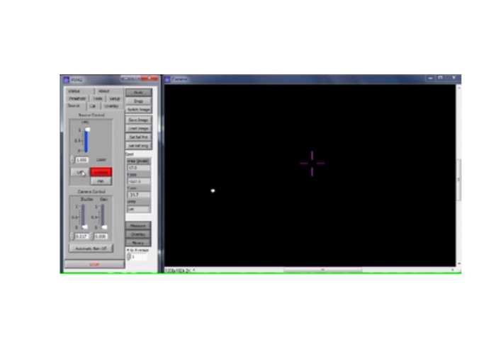
IN FOCUS BUT DECENTERED COFC SPOT
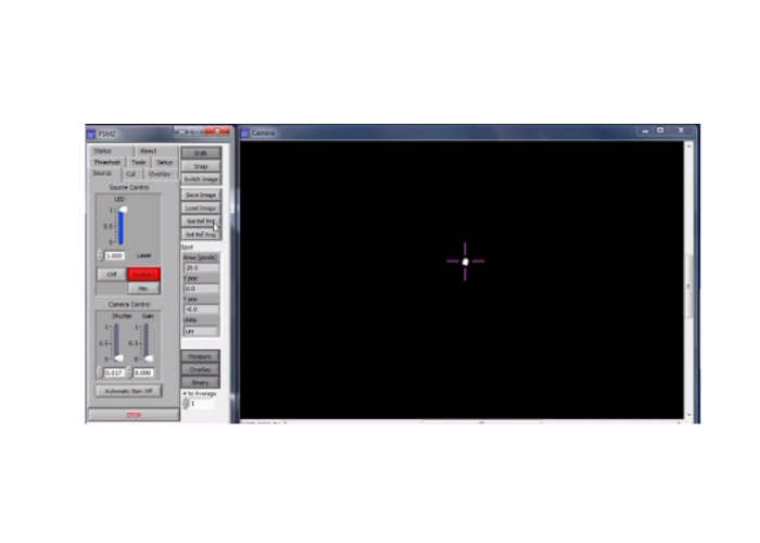
IN FOCUS AND CENTERED COFC SPOT
MEASUREMENT OF RADIUS OF CURVATURE
CONSISTS OF THREE STEPS:
Focus on the concave mirror surface to get a Cat’s eye reflection Set the reticle or electronic cross hairs on the reflected point image This established the optical axis of the ASM
Move the ASM back to near the center of curvature of the concave mirror Locate the reflected focused spot which may not be aligned to the objective Tilt the mirror until the reflected focused spot enters the objective Focus the ASM on the reflected spot and center it on the crosshairs Note the distance of the ASM on a linear scale
Move the ASM forward until it is focused on the mirror surface Moving from center of curvature means moving on a normal to the surface Get a sharp focus the Cat’s eye reflection Cat’s eye reflection will necessarily be centered on the cross hairs Read the distance of the ASM on the linear scale The difference of the Cat’s eye and confocal positions is the radius of curvature of the mirror
MEASUREMENT OF RADIUS OF CURVATURE
Focus on surface, used Cat’s eye reflection to set crosshairs
Move to confocal, adjust microscope so reflected spot in focus and centered on crosshairs, note linear scale reading
Move to focus on surface and get well focused Cat’s eye spot. Note scale reading Difference in readings is the radius of curvature
If this concept is well understood all other applications are easy
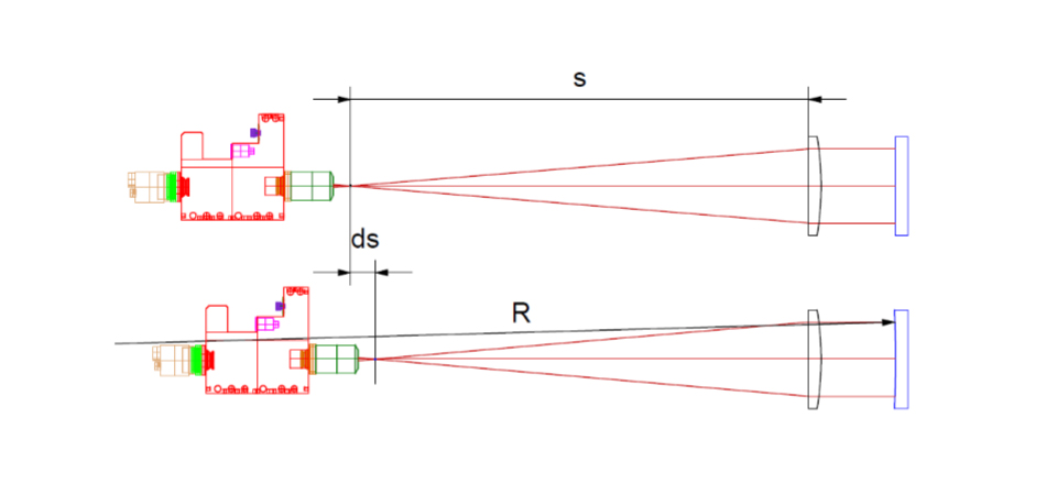
MEASUREMENT OF LONG RADIUS OF CURVATURE USE DEFOCUSED COLLIMATOR
Find s by putting a plane mirror in front of collimator
Put long radius surface in front of collimator and note ds
Since to first order efl = s, 1/s = 1/(s – ds) + 1/R, we find R = -s(1 + (s/ds)) (Be careful of signs, use common sense)
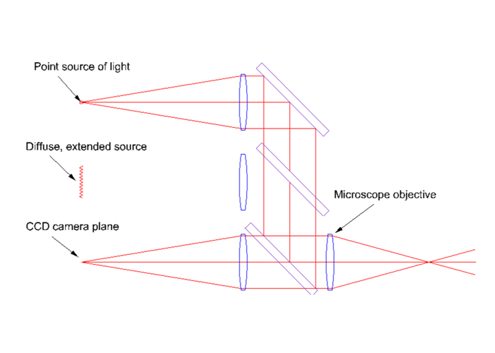
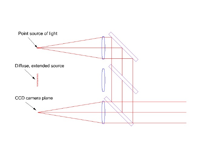
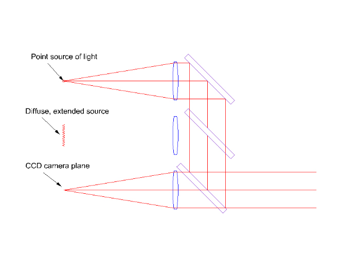
A CONTEMPORARY VERSION OF THE ASM IS THREE INSTRUMENTS IN ONE
Autostigmatic microscope
Internal SM fiber source
Electronic autocollimator
Simply remove objective
Video imaging microscope
Image plane parafocal with ASM focus
Internal LED Kohler source
SOME ADVANTAGES OF THE CONTEMPORARY DESIGN
Use of solid state light sources – compact, internal, low heat, monochromatic SM fiber coupled laser diode – bright for ease of alignment, near perfect spot Video camera – ergonomic, high position sensitivity, settable reference Software – permits high resolution centroiding on reflected spot
Large dynamic range on reflected light intensities
Recording and storage of Star images for optical quality determination
Centroid data easily coupled into other scales, a CMM, for example
OTHER USES OF THE ASM; DESIGNED FOR ALIGNMENT
Perfect for locating centers of curvature and foci of optical systems Use as a sensor on a centering station using a rotary table to define an axisUse was to align the elements of a f-theta laser scanner lens to a common axis Lens system had spherical and toroidal lenses and an “off-axis” mirror ASM mounted to the ram of a coordinate measuring machine Used a large x, y, z stage to pick up centers of curvature and align to axis
Don’t think like a lens designer and where rays go
Think about where centers of curvature should go and how to get them on a common axis
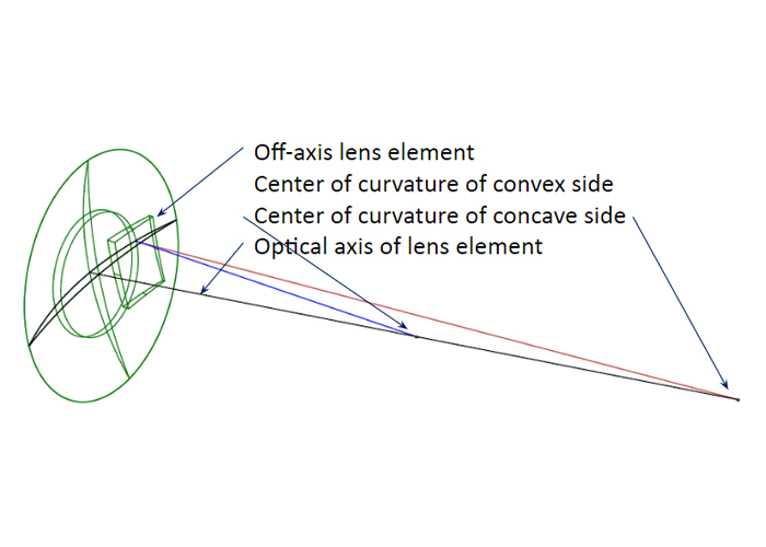
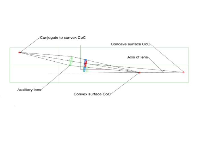
USE TWO ASM’S TO ALIGN AN “OFF-AXIS” LENS
Radius of convex side longer than working distance of objective, need extra lens
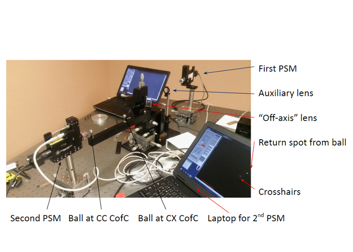
SET-UP USING 2 ASM’S TO ALIGN LENS
ALIGNMENT OF FOLD MIRRORS
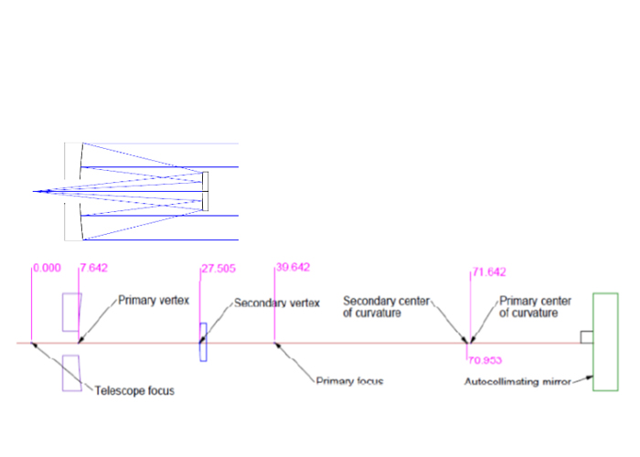
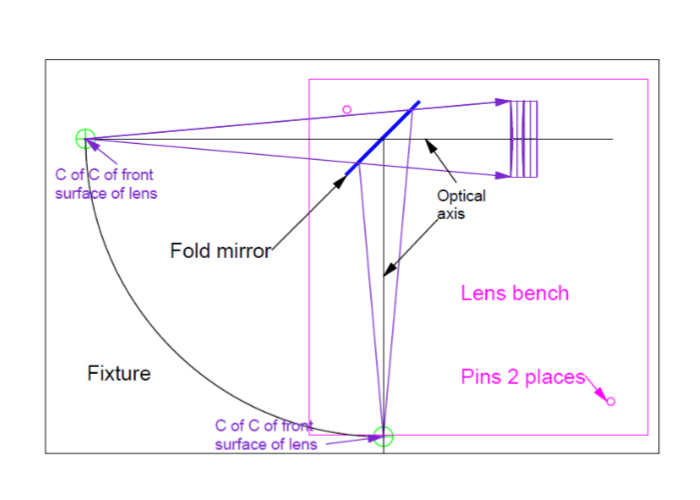
Plane fold mirrors have 3 degrees of freedom, 2 tilt and one displacement< Optical and mechanical design will show where the center of curvature should be located when the fold mirror is proper aligned A ball in a fixture will mechanically locate this position, and ASM can verify
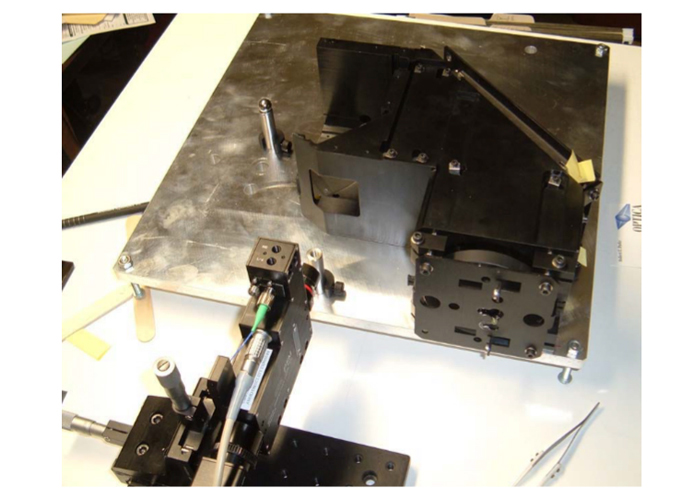
ANOTHER EXAMPLE OF A FIXTURE FOR ALIGNMENT
THE ROLE OF STEEL BALLS IN ALIGNMENT
Steel balls are a physical realization of a point in space Something you can physically touch as opposed to a theoretical object The ball center, the “point”, defines 3 translational degrees of freedom in space The ASM transfers an optical point, a CofC or focus, something you cannot touch, to the center of a ball, something that can be located physically Steel balls are inexpensive, extremely precise and come in many sizes Grade 5 chrome steel balls are round to 125 nm and cost about $3 each Can be thought of as convex optical grade mirrors Plug gauges are the cylindrical equivalent of balls and define axes in 3 DofF (Plug gauges are Go/no go pins for gauging the size of holes)
ALIGNMENT USING ABERRATIONS
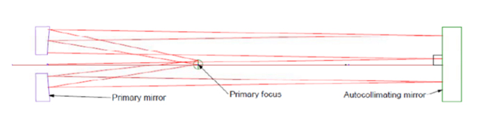
An ASM is a “Star” test device showing the point spread of an aberrated wavefront It has sensitivity to about lambda/8 or lambda/10 Useful for quick check of quality of optical surfaces as they are assembled into systems Alignment of a parabola as an example
Initially the return spot will not be centered on the crosshairs of the ASM The parabola or autocollimating mirror are tilted until return spot on crosshairs
ALIGNMENT USING ABERRATIONS (CON’T)
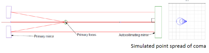
When return spot lies on the crosshairs, the rays strike the flat at normal incidence However, the normal to the flat may not be parallel to axis of parabola As a consequence, the return spot will show coma
To finish the alignment, tilt the flat while keeping return spot on the crosshairs until the coma is reduced to a symmetrical spot. The entire alignment process takes only minutes to accomplish
OTHER USES OF AN ASM – FINDING LENS CONJUGATES
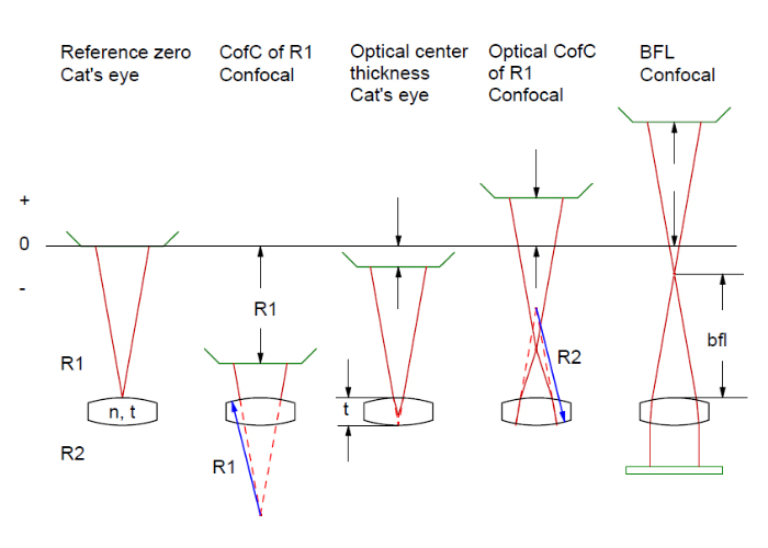
FINDING FIRST ORDER LENS CONJUGATES
Finding the radius of curvature of one side is direct measurement This assumes it is concave or there is sufficient working distance
Almost any lens can be reversed and measured through the side if not enough working distanceTo find the other conjugates it is necessary to model with a lens design program Or use first order equations and an iterative equation solving program See Parks, R. E., “Measuring the four paraxial…, Appl. Opts., 54, 9284 (2015)
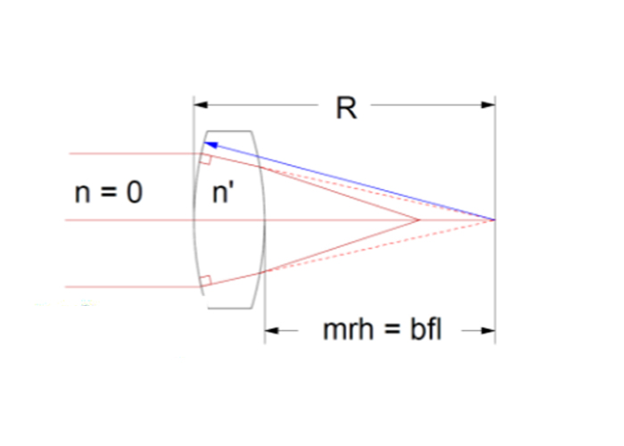
ZERO INDEX MATERIAL – A USEFUL TRICK
When using an ASM or an interferometer most setups are double pass Light comes from the instrument, reflects at normal incidence off the last surface and retraces itself back into the instrument For a quick insight to the test it is a lot of work to trace a double pass system The trick; reverse the system and make rays leave the last surface at normal incidence To do this have rays from infinity travel through a medium of 0 index to the last surface Then n*sin(θ) = n’*sin(θ’) = 0, so θ’ = 0, or the rays leave the last surface normal to it! Now a marginal ray height solve after the last refraction shows the paraxial focus
Credit for the idea; I don’t know who deserves it I learned it from Jim Burge at UofA, Optical Sciences I suspect he may have learned it from Roland Shack If someone knows a better attribution I like to know.
AN EXAMPLE – FINDING COFC’S AND SURFACES
Assume a simple optical system such as an air spaced doublet Find the centers of curvature and surfaces vertices looking into the system
Reverse elements, object at infinity and n = 0, float by stop on last surface
MRH = 26.403 = 24.395 = 39.445 = -94.453 Object on first surface, image space f/# large, stop on last surface
MRH = -7.471 = -5.492 = -3.368 = 0
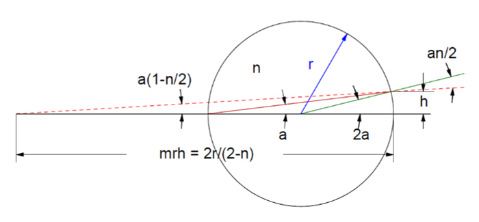
FIND THE INDEX OF REFRACTION OF A BALL
For small angles a = h/2r, and the normal = 2a, so the refracted ray angle is an/2 The ray angle relative to the x axis is 2a – an/2 = a(1-n/2) The mrh = h/(h/r(1-n/2)) = 2r/(2-n)
Or, n = 2(mrh – r)/mrh Works even if ball behind a window in a thermal chamber, but use ray trace
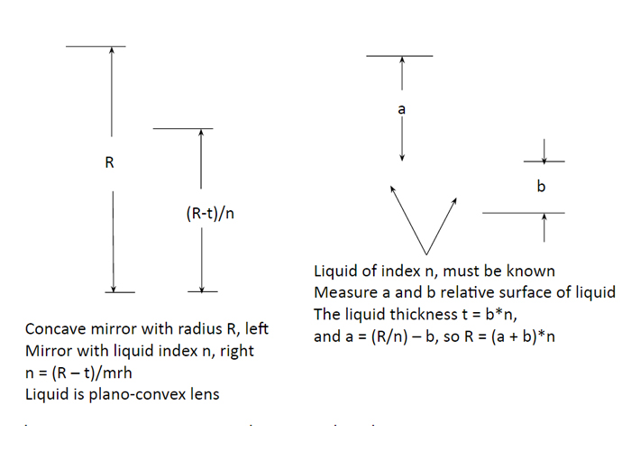
FIND THE INDEX OF A LIQUID AND RADIUS OF A SUBMERGED SURFACE
MEASUREMENT OF ANGLE
As shown earlier, by simply removing the objective the ASM is an autocollimator with sub-arc second sensitivity The bright mode of the laser source makes initial alignment easy in ambient light The small beam size makes it particularly useful for inspecting small prisms
ASM’S AND COMPUTER GENERATED HOLOGRAMS
A CGH pattern can simulate a ball, that is focus light a specific distance above the CGH
If balls are used to kinematically locate a CGH, a pattern to locate the balls can be included as part of the overall pattern. Then an ASM can precisely locate the balls. The balls, cemented in place, become an integral part of the CGH test artifact.
Because a CGH pattern can simulate a ball, a CGH can be made as an artifact for locating a group of points in space precisely located to < 1 μm in 3 dimensions.
An ASM mounted on a robot arm, for example, could be used to pick up the points one at a time to train and calibrate the robot.
EXAMPLE OF CGH HOLOGRAM
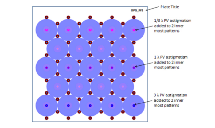
Printed on a 150 mm square photomask substrate Each circular pattern produces points several distances above the CGH Actual photograph is not available at the moment CGH courtesy of Arizona Optical Metrology, LLC, www.cghnulls.com
CONCLUSIONS
While autostigmatic microscopes (ASM) are over 100 years old, modern technology makes them truly practical for many diverse optical metrology needs.
Once the basic operation of measuring the radius of curvature with an ASM is understood, it becomes obvious that an ASM has many more useful applications.
Almost everything discussed here can also be done with an interferometer with greater precision. However, if the ultimate in precision is not needed the ASM is more convenient to use because of its small size, light weight and ease of mounting. Further, in some applications the greater coherence of an interferometer make some of the applications more difficult to perform because of multiple fringe patterns.
In many instances an ASM is a cost effective and easy to use alternative to an interferometer.
Could measure physically, but may not want to, or can’t
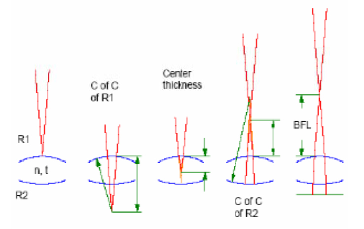
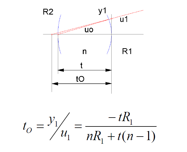
Measurements needed
Radius of curvature but may not have working distance – reverse lens so backside concave
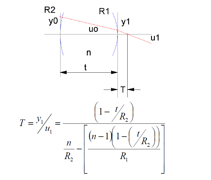
Optical center thickness to rear vertex
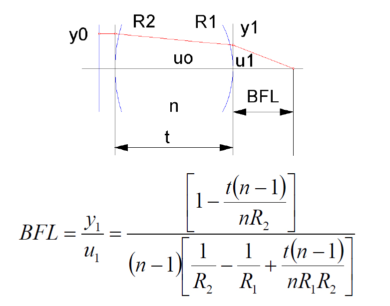
Back focal length from one or both sides
Need at least 4 measurements to solve for 4 unknowns
Extra measurements increase confidence
Measurements that can be made
Center thickness
Rear Radius
Back focal length
No closed form solution for unknowns
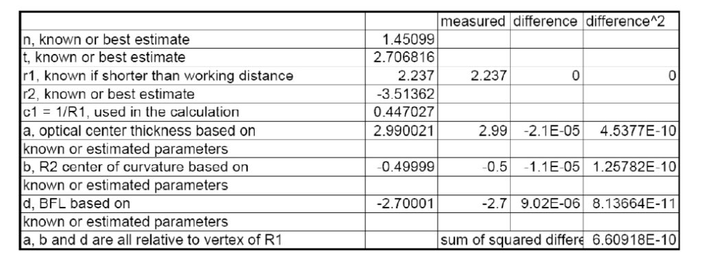
Use spreadsheet
Find difference between measured & guessed values
Square differences and sum
Make sum zero by varying unknowns
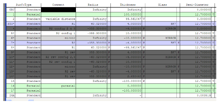
Use a lens design program
Model the various measurement configurations
Use multi-configuration option
Use plane surfaces, guess thickness and a model for index
Use optimizer to find solution
Spreadsheet example
N, t and r2 were estimated and a, b and c calculated
Solver used to minimize lower right hand cell to give calculated n, t and r2 shown above.
Lens design example
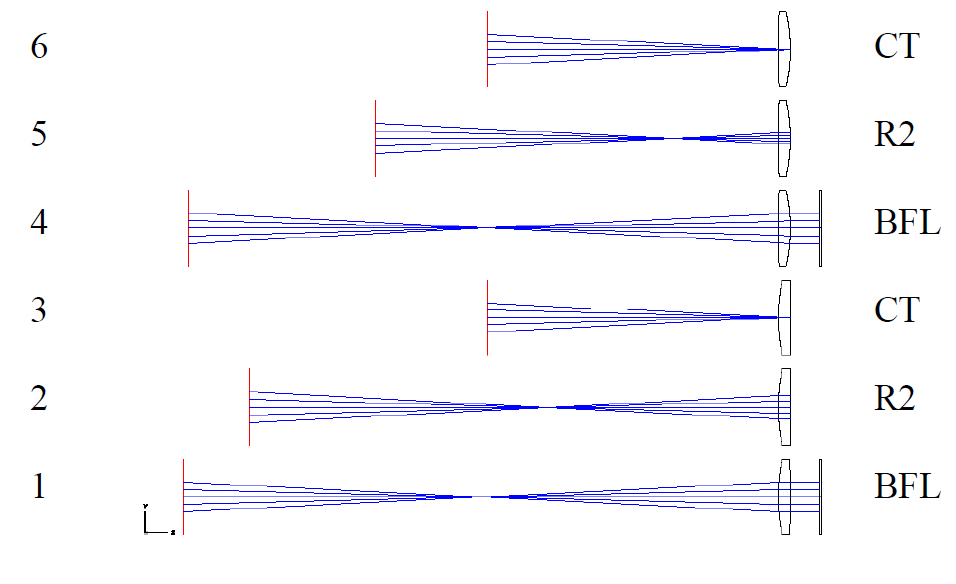
Configuration 1 shown for calculation of bfl
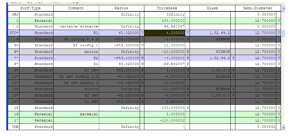
Grayed out lines are ignored
Lens design example con’t 1
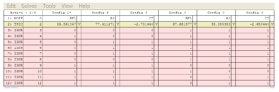
Configurations 1, 2 and 3 are looking thru short radius first Configurations 4,5 and 6 are looking thru long radius first Line 2 shows what the measurements should be knowing the index, thickness and two radii
Lens design example con’t 2
Lens design example con’t 3
Radii, thickness and index are set as variables
Optimized with small entrance pupil for paraxial solution
Conclusions
Use all practical conjugate measurements in model
Works with interferometer or autostigmatic microscope