Practical Alignment Using An Autostigmatic Microscope

ABSTRACT

Auto-stigmatic microscopes (ASM) are useful for bringing centers of curvatures of lenses and mirrors to the centers of balls used as part of an alignment fixture. However, setting up the fixture to get the balls used for alignment in a straight line to represent the optical axis generally requires another piece of equipment. We show that within a practical range, the autocollimation mode of a modern ASM can be used to align balls to an axis with about the same precision as they could be aligned with an alignment telescope, or laser tracker. As a lead in to this topic, we discuss our meaning of alignment, the means of positioning optically important features such as centers of curvature and foci to the coordinates specified on assembly drawings. Finally, we show a method of using an ASM along with other tooling to align a toroidal mirror using its foci.

1. INTRODUCTION

1.1 Definition of alignment

In a paper on alignment we should start by defining alignment. Every optical system is built to a design. First, there is the optical design, and it is used by a mechanical engineer to design a barrel or optical bench into which the lenses and mirrors are held. Throughout this design effort, the optical elements are assumed precisely located where the design specifies. It isn’t until the optical bench and elements come together that the issue of alignment comes up. It is at the assembly stage where the elements must be located precisely where the design or drawing specifies. This is alignment, getting optical features such as centers of curvature, axes, and foci positioned precisely as the design or drawing indicates.

In order to get the optical features located precisely, an instrument is needed that can sense the optical feature in question precisely. The same instrument, in conjunction with mechanical tooling, must also sense mechanical datums in the lens barrel or optical bench since the axes and foci of the optical system must be positioned precisely relative to specific mechanical features called out in the design. For example, the design may call for the optical axis of a system to be concentric with the outside of the cylindrical barrel of the assembly. Thus there must be a way of locating both the optical axis of the optical elements and the mechanical axis of the cylindrical barrel to assure coincidence of the axes.

1.2 Autostigmatic microscope

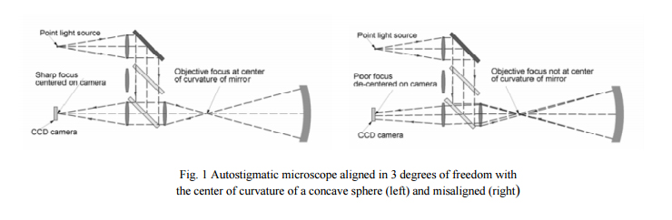
An instrument that can define both optical and mechanical datums in conjunction with some simple mechanical tooling is an autostigmatic microscope1 . In simplest terms, an autostigmatic microscope is a microscope that has a point source of illumination that is conjugate with a set of crosshairs in the image plane, either real physical crosshairs in an eyepiece or electronic crosshairs on a video display. If the autostigmatic microscope is perfectly aligned to the center of curvature of a sphere, the reflection from the sphere will form a well focused point image centered on the crosshair, that is, it defines 3 degrees of freedom (DOF). If the microscope is not well aligned the spot will be out of focus and shifted laterally from the crosshairs. Fig. 1 shows the typical optics of an autostigmatic microscope both aligned and misaligned with a concave sphere.

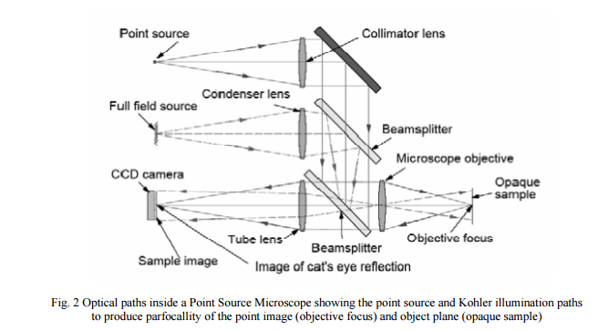
In order to make the autostigmatic microscope more useful, the addition of full field, or Kohler, illumination is helpful so the microscope can image as an ordinary microscope does. If the focal plane of the imaging arm and the autostigmatic focus are the same, the instrument is even more useful in that both types of illumination can be used simultaneously as will be illustrated in the first example of its use in section 2. A microscope with these features that is commercially available is called a Point Source Microscope2 and the optical paths in the microscope are shown in Fig. 2.

2. ALIGNMENT OF A STAGE COINCIDENT WITH AN AXIS OF ROTATION

2.1 Some definitions

As a first example of alignment with an autostigmatic microscope, we will consider the alignment of a single axis linear stage with the axis of a rotary bearing. The specific example will be a vertical stage over a rotary table used for centering lenses, but the example is just as applicable to the alignment of a lathe headstock with the lathe bed and tailstock center.

As with the term alignment, it is best to start with a definition or two. Since we are aligning an axis we should note that an axis is a line and a line is defined by two points, or a point and an angle in two planes, in other words by four DOF. Rotation about the axis and distance along the axis are not defined.

Another term used in conjunction with axes of rotation is centering and this can be confusing since there can be two meanings to centered. For a point, or spot, to be centered on an axis of rotation it is stationary when the axis is rotated. For the axis to be centered on the microscope, the axis must lie on the microscope axis, or crosshairs. The illustration in Fig. 3 helps explain the difference in the two concepts assuming a rotating table.

In the upper left of Fig. 3 the spots of light produced by the autostigmatic microscope move in a circle as the rotary table revolves about its axis. This means the light spot does not lie on the axis of rotation. In the lower left, the light spot is centered on the axis of rotation, but the axis of rotation is not centered on the microscope axis, or crosshairs. In contrast on the upper right, the spots are rotating about the microscope axis but are not centered on the axis of rotation, while in the lower right, the spots are both centered on the axis of rotation and that axis is centered on the microscope axis or crosshairs. In short, if the spots are moving in a circle, the spots are not centered on the axis of rotation meaning the center of curvature from which the spots are reflecting does not lie on the axis of rotation of the rotary table.

The same concept applies to centering an object in the microscope field of view. Consider the crosshair target in Fig. 4 that is imaged by the microscope. One end of the crosshair is indicated by a circle to show that the crosshair rotates as its center traces out a circle about the axis of rotation of the rotary table.

As seen in the lower left view of Fig. 4, the crosshair will rotate as the axis is rotated but the center of the crosshair remains stationary in the field of the microscope indicating that the crosshair lies on the axis of rotation but is not centered on the axis of the microscope while it is in the lower right view. The two types of centering require two physically different operations; to center the spots or crosshair on the axis of rotation, the optical surface must be translated or tilted relative to the axis of rotation. To get the axis of rotation to lie on the microscope axis either the microscope must be moved to the axis, or the axis of rotation translated or tilted to make it coincident with the microscope axis or crosshair.

2.2 Alignment of an axis

Now to the alignment of the vertical stage to the axis of the rotary table. Fig. 5 illustrates the situation. There is a rotary table in the lower part of the Figure and a vertical stage to the right. The Point Source Microscope (PSM) is shown in two positions on the stage, one focused on a target on the table using the imaging light source and one at the center of curvature of the plano concave lens lying on the table. These two foci of the PSM are the two points on the line defining the axis of the stage since the PSM is physically tied to the stage. The axis of the table is virtual because it cannot been seen, but it is made real by use of two simple fixtures, a crosshair target on the rotating table defining one point on the axis and the plano convex lens defining the other.

To align the axis of the rotary table to the axis of the stage as defined by the PSM focus, we must both make the target crosshair and the reflection from the concave surface stand still in space. This is accomplished by translating the target and lens, separately, relative to the table top. The target can be a piece of paper with the lens sitting on top. When the PSM in the imaging mode is focused on the paper the situation will typically look like the case in the upper left of Fig. 4. The target must be decentered relative to the rotary table top until it looks like the case in the lower left of Fig. 4. Then the target crosshair lies on the axis on the rotary table.

Similarly, at the center of curvature of the lens, the situation will look like the case in the upper left of Fig. 3 when the PSM is focused at the center of curvature using the autostigmatic mode. If the vertical stage is very decentered, the stage may have to be translated to get the return image in the field of view of the microscope, but the real task is to make the reflected spot cease to move as the table is rotated, that is, to achieve the case shown in the lower left of Fig. 3.

Once the crosshair and spot are centered, that is, not moving except in the case of the cross, rotating about the center of the cross, it is then necessary to translate and tilt the stage until the cross and spot both lie on the crosshairs in the microscope. When the alignment is finished the crosshair target will look like the case in the lower right of Fig. 4 and the spot will look like the lower right of Fig. 3. It is important to make these adjustments in the correct order, center the targets on the rotary axis first and then adjust the column. Further, remember that the target errors are seen doubled due to the rotation, and in the case of the spot, reflection. Do not try to make the full correction all at once. You will overshoot every time and the alignment will take at least twice the time it should. Make the adjustments in fractions of what it looks like the translation needs to be.

Notice, too, this alignment could not be done without some simple fixturing to “realize” datums that are virtual without the fixturing. In general, the most useful fixtures are spherical surfaces, physical realizations of points, and next most cylinders, realizations of lines. These make the most precise realizations because if lens surfaces or high grade spherical balls are used, their centers can be located to <1 μm. With images of crosshairs, it is difficult to use centroiding algorithms to achieve micron centering, but 10 μm centering is easy with images.

3. ESTABLISHING AN AXIS

In this example, we will describe how to use an infinity conjugate autostigmatic microscope to establish an axis. This is important because the majority of optical systems have a single axis of symmetry and alignment for these systems means having the centers of curvatures all lying on a common axis. In passing, the easiest way of establishing an axis is to use a good rotary bearing like in the previous example. However, there are many times when such a table is not available or the optics are too large to put on a rotary table.

For the alignment of a system with a single axis, fixtures or datums have to be positioned at precise locations along the axis. The lateral positions are tighter than the axial locations, but the axial locations still need to be carefully controlled. The most common way to do this alignment is with an alignment telescope3 , but it is a tedious proposition and almost always requires two people, one looking in the eyepiece and one making the adjustments to the fixtures.

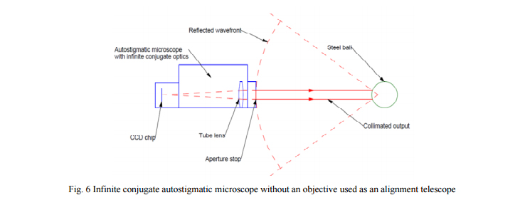
There is an alternative that works well over distances from about 0.5 m to 3 m. That is, remove the objective from the autostigmatic microscope and use the collimated beam projected by the 6 mm aperture. When the collimated beam reflects off a spherical surface, the return wavefront is nearly spherical, and for that part of the wavefront returning through the aperture on the microscope it is perfectly spherical assuming a good grade spherical ball. This situation is like that shown in Fig. 6 where a steel ball is used to maximize the reflected light.

The spherical wavefront reflected off the ball will have a radius of curvature of approximately the distance from the microscope to the ball. Assume for this example the distance is 1 m and the ball is 25 mm in diameter. The PSM has a 6 mm aperture and a 100 mm tube lens. This means the return wavefront will produce a spot about 0.6 mm on the 1/3” CCD detector that is 3.6 mm in the short direction. While this is not a perfectly focused spot, the centroiding algorithm in the PSM software works just as well on out of focus images as well focused ones. The limit here is that the entire spot lie on the CCD. In this example, the shortest distance from ball to PSM would be 250 mm to keep the image from being bigger than the detector. If a shorter distance were needed, the 6 mm aperture could be stopped down. Also, short distances mean plenty of light gets back through the aperture stop.

The far distance is limited by the light available but has the advantage that the spot on the CCD is smaller. For the example, the 6 mm collimated beam is spread into a cone of 0.235 steradians. At a 1 m distance, the 6 mm aperture subtends just 36 μsteradians, or collects just 1.5×10-4 of the reflected light assuming a top hat intensity distribution. On the other hand, the PSM has an intensity dynamic range of about 1×105 . Thus a dynamic range at a distance of 3 m or more is perfectly reasonable.

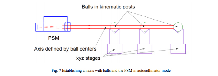
Figure 7 shows the PSM used in the autocollimator mode to align a set of balls on a common axis. Here the farthest ball is aligned first. A post such as used to position lens mounts can be used as a kinematic locator for the ball. The post is on an xyz stage and the stage is adjusted until the reflection from the ball is centered on the PSM display. Subsequent balls are similarly adjusted. The axial spacing is set using an inside micrometer.

There are several advantages over using an alignment telescope in addition to those already mentioned. The collimated beam is bright enough to see under ambient lighting so it is easy to set up the initial alignment, the balls are easier to use than crosshair targets needed with an alignment telescope, the set up has no moving parts in the alignment instrument and there is nothing to focus. Finally, the centroiding is completely objective.

In terms of precision, the centroiding algorithm has a sensitivity of just under 1 arc second, or ~5 μradians. Even with out of focus images on the detector experience has shown this to be the case. The means that balls aligned using this method can be positioned to about ±5 microns at the distance of 1 m. Over the range where sufficient light reaches the detector this sort of precise is on the order of that achievable with a laser tracker.

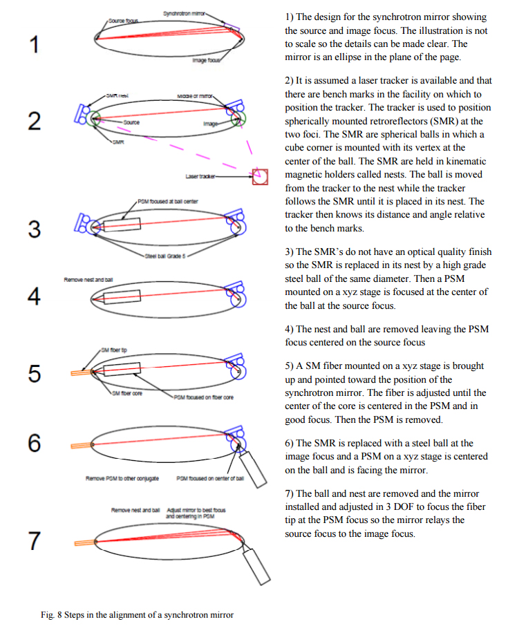
4. ALIGNMENT OF SYNCHROTRON MIRRORS

The final example is one that I have not had the opportunity to try out but is illustrative of a technique that could be applied to many situations where high precision alignment is required in a multi-dimensional space. Further, it shows how the autostigmatic microscope can be used along with other sophisticated optical tooling such as a laser tracker4 to increase the value of both the tracker and the microscope. The whole example is laid out in Fig. 8 and the various steps will be described in the text, one after the other. This is again an example of how there is a particular sequence of steps that must be gone through to achieve the final alignment.

The synchrotron mirror is⁵ almost plane and thus has the same DOF as a plane mirror, rotation about the axes parallel to its face and translation perpendicular to its face. Using these 3 DOF the mirror is adjusted so the light from the fiber tip is focused at the PSM focus. The focus will be a line normal to the page and have a width limited by diffraction set by the apparent width of the mirror looking into it at grazing incidence in the plane of the page. The other 3 DOF are set using mechanical datums on the mirror and the structure holding the mirror.

In this example we have tried to demonstrate the use of the autostigmatic microscope with other optical tooling used in large optical projects. The SMR’s used by the laser tracker are completely compatible with the use of steel balls used in other autostigmatic microscope applications. The imaging aspect of the PSM permits its use in the location and centering of an optical fiber tip that will then be used as a point light source at one conjugate of the system. Finally, the PSM can be used to detect the focused image coming single pass through the optical system to align the synchrotron mirror.

5. CONCLUSIONS

We have first set out a working definition of optical alignment as determining the location of an optical, as opposed to a mechanical, feature, and then moving that feature to the location specified in the design of the optical system. Then we have given a simple example of the alignment of a center of curvature to an axis of rotation to show the difference between alignment of the feature to the axis of rotation, and the alignment of the axis to the instrument making the measurement. This is followed by an example of using an infinite conjugate autostigmatic microscope to align a series of spherical ball targets in a straight line. Finally, we show how to use an autostigmatic microscope in conjunction with a laser tracker to systematically align a synchrotron mirror using the mirror’s two foci.

REFERENCES

[1] Steel, W. H., “The Autostigmatic Microscope”, Optics and Lasers in Engineering 4(4), 217-227 (1983).
[2] www.optiper.com
[3] For example, http://www.brunson.us/p/AboutAlignTel.asp
[4] For example, http://www.faro.com/laser-tracker
[5] http://www.bnl.gov/nsls2/project/CDR/Ch_08_Radiation_Sources.pdf, p. 18.