Calculation Of The Vertex Radius Of An Off Axis Parabolic Surface Using The Sag Measured With A Three Ball Spherometer

Abstract

We describe a method of calculating the vertex radius of an off-axis parabolic segment using a three ball spherometer to measure the sag. The vertex radius is found by solving a set of six simultaneous, non-linear equations for the three coordinates of one of the ball centers and the corresponding three coordinates of the point of tangency of the ball with the surface.

1. Introduction

Three ball spherometers are the 1” micrometers of an optical shop and have been used for over 100 years to measure the radii of spherical surfaces.^1,2 The radius of curvature of a spherical surface can be calculated from a simple, three term formula that includes the measured sagitta, or sag, the distance from the central micrometer or indicator and the center of the balls and the radius of the balls.^3,4 Until recently, in spite of the simplicity of the formula that includes a square in one term, spherometers were sold with tables that converted sag readings into radii because optical shop personnel often did not have the skills or time to solve the formula. With the advent of pocket calculators it is now easy to solve the sag equation.

The sag equation is rather simple because the spherometer balls touch the surface at normals to the surface, and for a sphere these go through the center of curvature of the sphere and through the centers of the balls on the spherometer. In the case of an aspheric surface this is not so; the ball centers still lie on the normals to the aspheric surface but the normals do not go through the center of curvature of the asphere. The solution to this problem requires the solution of six non-linear, simultaneous equations, again something not easily undertaken even by rather mathematically adept optical engineers. However, with the advent of equation solvers such as the “Solver” function in Microsoft Excel, solution of these simultaneous equations is straight forward and fast. This is the problem we will illustrate.

2. Measured surface sag (T)

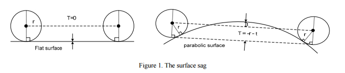
The measured sag, T, is the difference between the spherometer indicator reading when the spherometer is sitting on a plane surface, Fig. 1 (left), and when the spherometer is resting on the aspheric surface to be measured (right). We have shown the case for a convex surface but identical conditions hold for a concave surface with the exception that the sign of the indicator movement is opposite.

3. Geometry of the three ball spherometer

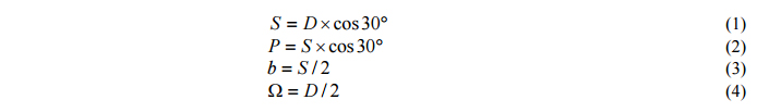
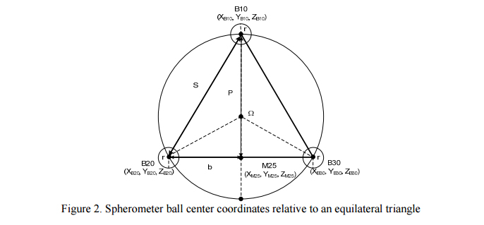
Referring to Figure 2, the spherometer has three balls on the points of an equilateral triangle. D is the diameter of the circle through the centers of the balls, S is the length of the side of the triangle and the distance between ball centers, P is the height of equilateral triangle, Ω the distance from the center of the triangle to the balls and r is the radius of the balls. B10 is the center of the ball located on the meridional plane of the parabolic segment and the vertex of the parabola lies above this ball. B20 and B30 are ball centers located symmetrically with respect to the meridional plane. Relationships of the sides of the spherometer are given below.

4. Geometry of the spherometer resting on the parabolic surface

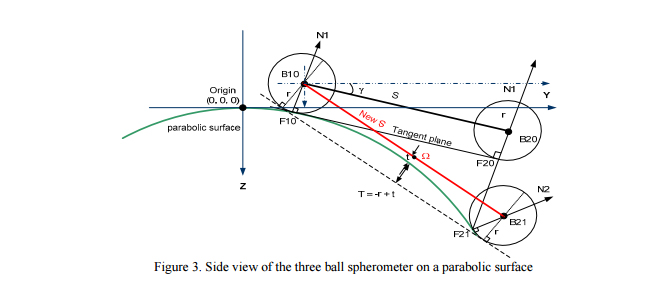
We use a Cartesian coordinate system where z is the axis of symmetry of the paraboloid and y lies in the meridian plane. The origin is coincident with the vertex of the parent parabolic surface. When the spherometer is first set on the parabolic segment we place ball B10 on the meridional plane with the tip of the indicator approximately centered on the segment. At first we know only that X_B10 = 0, Y_B10 is approximately P less than the center of the segment and Z_B10 is r higher along the normal to the surface than where the ball touches the surface, Z_F10 = Y_B10^2/(2R_v) where R_v is the vertex radius of the parabola.

Referring to Fig. 3 we see the spherometer in two states, the final one (subscript 1) sitting on the surface and an initial one (subscript 0) where the calculation is begun. We start by assuming the plane of the three spherometer balls is perpendicular to the normal to the surface at F10. This allows us to calculate a starting position for B20, and by shifting the plane of the ball centers downward by r, the starting position for F20.

Then we assume the spherometer is iteratively rotated down to the surface about the center of B10. The point of contact, F10, will not change nor will the dimensions of the spherometer. However, as the spherometer is rotated so the other two balls rest on the surface the calculated dimensions of the spherometer will change. Since the spherometer dimensions cannot change we have a method of solution by simultaneously solving the six equations below for the centers and points of tangency of the floating balls.

5. Calculation of points of tangency to the parabolic surface of the equilateral triangle base

The six unknown variables are

and they are found by solving six equations simultaneously. The six equations are

The relationship of the ball center to the point of tangency along the normal to the surface

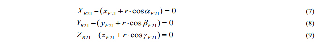
where α, β and γ are the angles of the normals to the surface at F21. Finally the distances between the balls

Once the six unknowns are found it is straight forward to find the coordinates of the center of the spherometer and project the indicator down to the surface of the parabolic segment normal to the plane of the ball centers. In general, the tip of the indicator will not hit the center of the segment exactly and a new value will have to be used for Y_B10 and the calculation repeated until the tip is close enough to the desired location. Notice too that we have calculated the sag assuming the vertex radius is correct. If the measured sag is different from the desired, the R_v in eq. 5 must be changed until the results match the measured sag.

6. Summary

We have shown how the sag of an off-axis parabolic segment as measured with a three ball spherometer may be used to determine the vertex radius of the segment. While this is not as easy as for a spherical surface, the calculation is well within the capabilities of an optical engineer with access to iterative equation solving software.

7. References

1. Grubb, H., Nature, 34, 85 (1886)

2. Ritchey, G. W., Smithsonian Contributions to Knowledge, 34 (1904)

3. Horne, D. F., “Optical Production Technology”, p. 324, Crane, Russak & Co., Inc., New York 1972

4. Malacala, D. “Optical Shop Testing”, p. 818, 3rd ed., Wiley-Interscience, 2007.