Author: csadmin

Prism Alignment Using A Point Source Microscope

Written by csadmin on June 28, 2019. Posted in PSM Applications, Published Papers. No Comments on Prism Alignment Using A Point Source Microscope

1. INTRODUCTION

Spherically mounted retroreflectors (SMRs) are an essential part of spatial metrology when using a laser tracker. However, the precision of the laser tracker measurement is no better than the precision with which the cube corner retroreflector is mounted in the spherical ball. Thus measuring the position of the apex of the cube corner with respect to the center of the ball is a critical part of both the assembly and inspection of SMRs. This leads to cost implications because the better centered the cube corner in the ball, the more the SMR costs.

We begin by explaining the use of SMRs with a laser tracker, and then explain how the question arose of whether an autostigmatic is useful in measuring the apex location of the cube corner. We follow this with the theory of the measurement based on a two-dimensional argument, but the same argument applies to the three-dimensional case. The two-dimensional case is much easier to explain and understand.

Finally, we look at how real hardware must be fixtured to make the measurements. At first it looks difficult because a sphere has no axis and the SMR must rotate about orthogonal axes to measure the apex location. However, a very simple fixture is satisfactory. We give some measured results to demonstrate the precision of the method.

2. USING SMRS

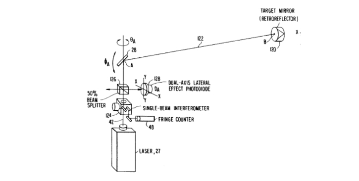
Fig. 1 is from US Patent 4,714,339 that describes a laser tracker. Light from a laser projects from a measuring head that rotates in azimuth and elevation. The light reflects back to the tracker from a target that is a cube corner retroreflector. There is a position-tracking sensor built into the head so the motorized azimuth and elevation axes follow the target and encoders on the axes record the angles versus a time base. In addition, there is a time of flight sensor that measures the distance to the target completely specifying the target position in a spherical coordinate system centered about the intersection of the azimuth and elevation axes of the head.

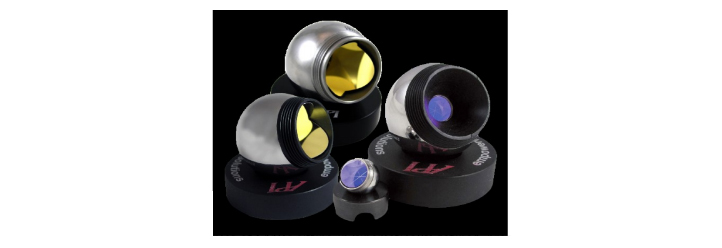
The cube corner retroreflector target mounts in a hollow ball such that its apex ideally sits at the center of the ball. The laser tracker metrology field calls this arrangement of a cube corner in a ball a spherically mounted retroreflector, or SMR. The SMR sits in a kinematic nest¹ attached to the structure being measured as shown in Fig. 2. The precision nest allows precise positioning to datums on the structure. Assuming a precise positioning of the nest, the SMR contributes an error to the measurement of twice the displacement of the apex to the center of the ball in all 3 degrees of translational freedom. Since laser trackers are capable of measurements in the range of a few μm’s and a few seconds of arc^2,3,4, the errors in the SMR contribute directly to the total error of the measurement.

3. PRECISE POSITIONING OF LASER TRACKER NESTS

Before discussing how we got into the measurement of the cube corner SMR, we should discuss the precise positioning of the SMR nests relative to datums on the structure the laser tracker interrogates. Because the SMR ball sits in the nest and balls are very easy to align precisely with an autostigmatic microscope (ASM)⁵, an ASM is an ideal method to help position nests. In all the cases we show in this paper, the ASM used was a Point Source Microscope (PSM)⁶, a convenient, modern version of a classic ASM.

Fig. 1. Diagram of a laser tracker from US Patent 4,714,339

Fig. 2. Examples of SMRs sitting in kinematically defined, precision “nests”

In one case, the test engineers wanted to know the location of a CCD camera image plane using a laser tracker since there was no convenient way to get to the camera during the actual test. A solution was attaching 3 nests to the exterior of the camera and using the PSM mounted on a precision stage to relate the nests, hence SMRs, to the image plane.

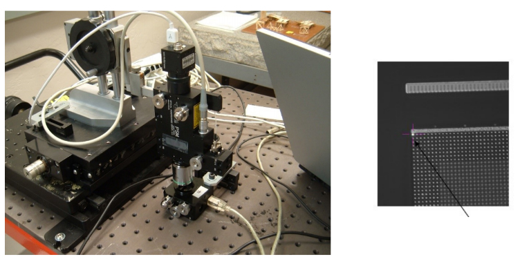
SMR balls come in standard sizes, one of which is 1⁄2”. By substituting full 1⁄2” balls for 1⁄2” SMRs it was simple to find the x,y,z positions of the centers of the 3 balls with the PSM. Then using the video mode of the PSM, the corners of the CCD array were located in the same coordinate system since the video image plane in the PSM is parfocal with the point source at the objective focus as in Fig. 3. This procedure tied the corners of the image plane to the 3 ball centers so that when SMRs were substituted for the solid balls, the laser tracker located the position of the CCD image plane. This is just one example of the use of the PSM to position SMR nests on the structure the laser tracker measures.

4. ORIGIN OF THE IDEA OF USING THE PSM TO MEASURE SMRS

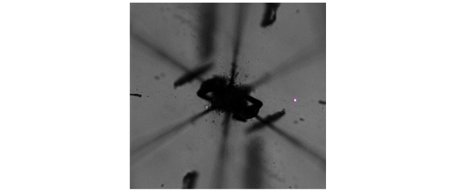
I was exhibiting the PSM at a trade show 2 years ago when a follow exhibitor came over and asked if the PSM could be used to locate the vertex of the cube corner relative to the center of the ball that held the cube corner. I had to admit I had never used the PSM to look into any kind of cube corner and did not know if the PSM would be useful. However, the question intrigued me and I set about looking for an answer. At first, it was not obvious whether the PSM should be used with a focused or collimated beam but since an objective was already installed that was tried first. When the microscope was focused down to the plane of the apex, a return reflection appeared mirrored across the apex from when the focused spot was incident. It was easy to see where the spot focused because the surfaces of the cube corner were illuminated with the LED source in the PSM while the point source was simultaneously illuminated as seen in Fig. 4.

Note that you cannot look right at the apex because it is not optically perfect and tends to collect contamination. This forces you to view the prism decentered from the apex. Then you to think the measurement cannot be made until you realize the corner reflector acts like a right angle prism and this behavior is exactly what you would expect in 2 dimensions. Now that it is clear some sort of measurement is possible, it is time to look at where the light rays are going.

Fig. 3. CCD camera with SMR nest attached to the camera body while the PSM is focused on the CCD array (right)

Fig. 4 Magnified image of the apex of a corner reflector with the PSM focus to the left of the apex and reflected spot to the right. The 6 pie segments of the reflector are obvious and as are contamination spots reflected across the apex.

5. IMAGING ON A SURFACE WITH A POINT SOURCE OF LIGHT

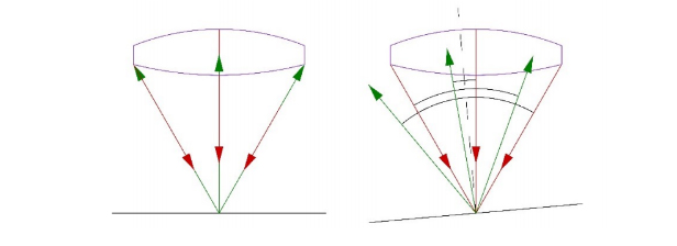
When a point source of light is imaged on a surface, we get a Cat’s eye, or retro, reflection as shown in Fig. 5. The rays incident (red) on the surface are reflected back (green) into the objective, obeying the part of the Fresnel law of reflection that says the angle of incidence equals the angle of reflection relative to the normal to the surface.

Fig. 5. A point source of light focused on a surface perpendicular and tilted with respect to the gut ray

As implied by the left picture, for every incident ray there is a reflected ray mirrored about the gut ray tracing the exact same path back into the objective lens of the microscope. The same holds when the surface tips with respect to the gut ray and center of the objective. Every incident ray reflects back into the objective mirrored about the normal to the surface, the black dotted line. The right hand picture makes it clear that not all the reflected rays make it back into the objective, nor is the surface uniformly illuminated about the normal so the reflected image appears oval, or football shaped, when viewed out of focus. The reflected spot appears round at exact best focus independent of tip.

The more important aspect of the tipped surface reflection is that the plane wave incident on the objective that creates the focused spot on the surface is parallel to the plane wave on reflection collimated by the objective. Fig. 5 implies this but it is not as obvious as the vignetting mentioned above. If a plane wave focused by an objective produces a spot at a specific location on a surface, then a point source of light in the same location on the surface projected toward the objective must produce a plane wave, once collimated by the objective, that parallels the plane wave originally producing the spot.

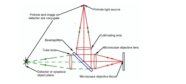
This property of the Cat’s eye, or retro, reflection is so obvious that we tend to overlook the implications, yet this is why an autostigmatic microscope is such a useful tool for aligning optics. We align the crosshair in the detector to the point source providing illumination to the surface through the objective by centroiding on the Cat’s eye reflection. The crosshair on the detector is then conjugate to the originating point source of light and to the focused spot on the surface as shown in Fig. 6.

Fig. 6. PSM ray diagram showing that the point source, its image at focus and its image on the detector are conjugate

The Cat’s eye image properties also include that the surface does not have to be plane or smooth. It is easy to obtain a Cat’s eye image off a ball or any spherical surface. At first, this seems counterintuitive but the focused sport is so small there is almost no change in the slope of the surface over the size of the spot so it behaves like a plane surface. While the best focused Cat’s eye images, in terms of a tightly focused spot, come from smooth or specular surfaces, it is easy to get a Cat’s eye from a piece of paper, for example. The spot will be larger in diameter than from a smooth surface, may be somewhat irregular in shape and will require greater source intensity to see, but will produce a spot with a minimum diameter at best focus that is conjugate to the point source of illumination.

We complete this analysis of the behavior of Cat’s eye images by going back to some geometrical definitions. Since one can pass a plane though a point it should come as no surprise that the plane can tilt around the point. Similarly, a spherical or cylindrical surface can pass through a point independent of the radius of either. These are the fundamental reasons for the behavior of a Cat’s eye image. All these properties are useful during initial alignment of test setups to get the various components roughly aligned and light back into the microscope objective for electronic video viewing.

6. AXIAL BEHAVIOR OF THE CAT’S EYE REFLECTION

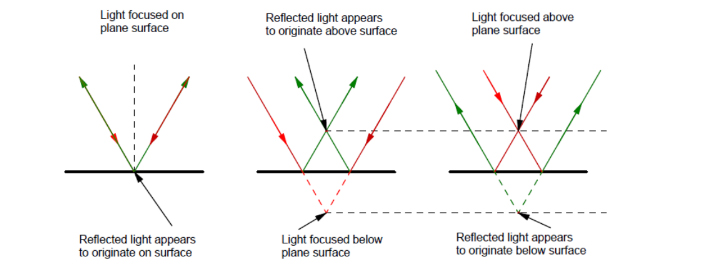
When the incident, focused spot is either above or below the surface when looking for a Cat’s eye image, the reflected spot looks like it is coming from below or above the surface, respectively, as seen in Fig. 6.

Fig. 6. Light focused above or below a surface appears mirrored in the surface axially

The incident (red) rays form a virtual focused image below the surface that produces a real reflected (green rays) image above the surface and vice versa. The dotted red and green rays are virtual.

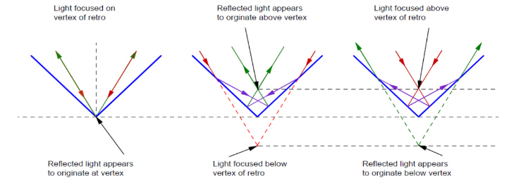
Fig. 7 shows the situation similar to Fig. 6 but this time looking into a hollow right angle reflector. This is a little harder to follow because of the extra bounce of light in the reflection but the net effect is the same as in the plane surface case, light focused below the apex looks like it is coming from above the apex, and vice versa. To make Fig. 7 a little easier to interpret the incident light is still red and the reflected green but the first reflection of the ray shows in violet. The horizontal dotted black lines show the distances above and below the apex while the colored dotted lines show the virtual rays.

Fig. 7. Light focused above or below a right angle reflector appears mirrored in the surface axially

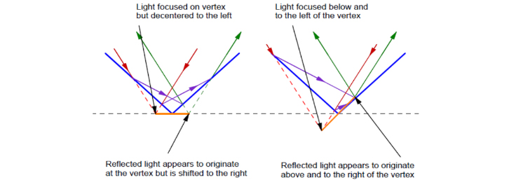
If the incident, focused spot is left or right of the apex but the same depth as the apex we have the situation in Fig. 8. This is different from a plane mirror that has no feature to create a symmetry. The apex of the hollow right angle reflector creates an axis of symmetry so that light incident to the left of the apex reflects the same distance from the apex to the right. The orange line shows the distance and orientation of the shift from the incident to the reflected virtual focus in the case (left) where the incident focus is the same depth as the apex. The situation gets more complex when the incident spot shifts laterally and axially. Again, the orange line shows the vector between the incident, and the reflected, virtual focus. The hollow reflector acts like a plane mirror to axial shifts but now has a symmetrical, lateral shift due to the axis created by the apex.

Fig. 8. Reflection from a right angle reflector where the focused incident light is not centered on the axis of the reflector (left) and not centered nor the same depth (right)

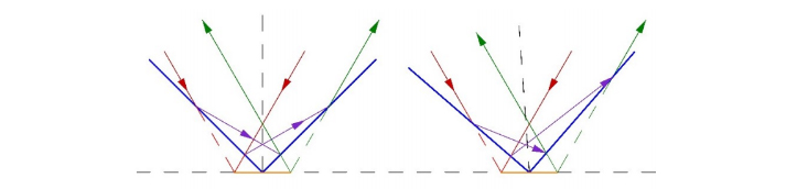
On the other hand, the hollow reflector behaves as expected when tipped about its apex and the incident light focuses at the same depth as the vertex. The lateral shift of the reflected spot does not change with tip of the reflector as seen in Fig. 9. This behavior suggests a method of finding the decenter of the apex. If the reflector turns 180 degrees but the apex is not on the axis of rotation then to the incident light the apex appears closer in one orientation than the other does. This means the reflected spot appears to move by twice the decenter of the axis of rotation from the apex.

Fig. 9. Reflection from a right angle reflector when the reflector angle bisector is parallel to the objective gut ray (right), or the reflector is tipped relative to the gut ray. (The tilt is slight so the Figure does not get too complex.)

7. MEASUREMENT OF APEX DECENTER

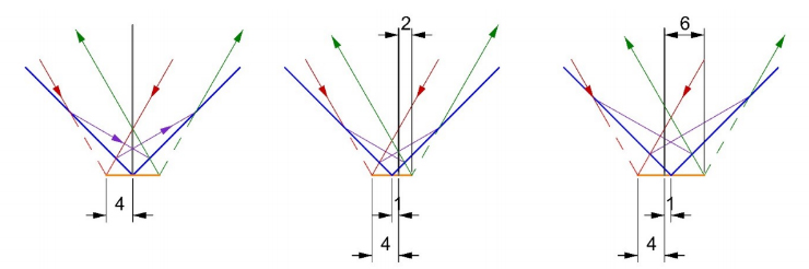
In Fig. 10, we show that if the reflector is rotated about an axis decentered 1 unit from the apex, the reflected spot moves 4 units laterally. In the picture on the left, the axis of rotation (heavy black line) is centered on the reflector apex and the incident focused spot is 4 units to the left is the apex. In the middle picture, the apex shifts 1 unit to the left of the axis of rotation but the spot is still 4 units from the axis of rotation. After rotating the reflector 180 degrees as in the right picture, the spot is still focused 4 units from the axis of rotation. Comparing the middle and right hand pictures, we see that the reflected spot moves from 2 units relative to the axis of rotation to 6 units upon rotation, or a 4x movement of the apex from the axis of rotation.

Fig. 10. Light incident 4 units from the apex (left), the reflector shifted 1 unit to the left (middle) and shifted 1 unit to the right by virtue of a 180° rotation about an axis 4 units from the incident spot.

We drew Fig. 10 using a CAD program to trace the rays but if you used algebra and trigonometry you would come to the same conclusion, as long as the incident spot is fixed relative to the axis of rotation, the reflected spot moves 4 times the decenter of the apex relative to axis of rotation. This is because the reflected spot is always symmetric with the incident spot about the apex. Because the apex shifts toward the incident spot in the middle picture, the reflected spot moves twice as much to the left. The opposite happens when the reflector is rotated 180 degrees.

8. BEHAVIOR WITH APEX ABOVE OR BELOW CENTER OF ROTATION

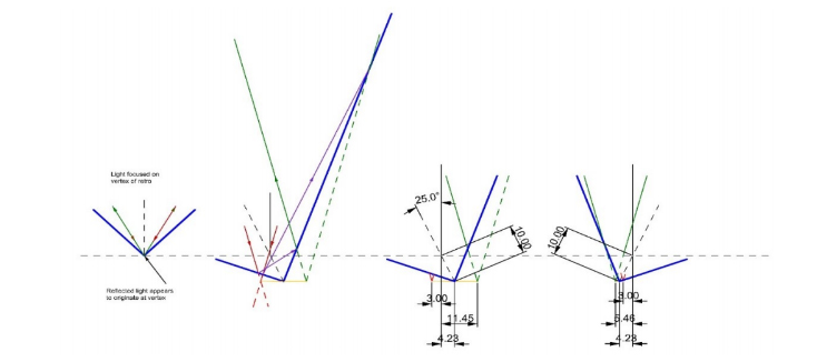
In order to find the distance between the apex of the reflector and the center of the ball, the SMR is rotated about the ball center. To get the maximum sensitivity the ball is tipped as far as possible without vignetting the beam, about 25- 30 degrees. It is difficult to draw a picture that clearly shows the true situation but Fig. 11 attempts to do so. If the beam focuses right at the apex the beam comes back upon it self. If the apex is below, or above, the center of the ball we have the case illustrated in Fig. 7 but the PSM precision is limited in the axial direction. If the ball is tilted about its center, the apex moves off the center of rotation so we have a situation somewhat like the decentered apex, and the reflected spot will shift laterally, a direction where the PSM has great sensitivity.

Fig. 11. Behavior of the reflected spot when the apex is below the center of rotation (3rd diagram) and after 180° rotation. The red and green dotted lines indicate the positions of the virtual images.

As seen in Fig. 7, if the PSM is not focused to the depth of the apex, the reflected spot will also be defocused. It is best practice to find best focus and then tip the SMR as far as possible without vignetting. Then we have the situation in the second picture of Fig. 11 where we have had to extend the reflector surface to show where the reflected ray is incident on the surface. This picture shows the overall ray paths and the bisector of the reflector faces. The bisector rotates about the ball center, the horizontal dotted line. The incident focused beam appears to reflect on the other side of the prism apex but at approximately the depth of the apex because this is where we focused the microscope.

The third and 4th pictures show more detail about the distances of the incident light and the apex that comes in at a fixed distance of 3 units from the center of the ball, or point of rotation. The apex shifts 4.23 units because this is 10*sin 25°. It is 7.235 units from the apex to the incident focus so the reflected focus is 7.235 units beyond the apex or 11.45 – 4.235. In the fourth picture, the ball was rotated 180° about a normal to the plane of incidence which moves the apex to the other side of the axis of rotation, in fact, beyond the incident focus. The reflected spot is still the same distance on the other side of the apex, 1.23 units on either side. Thus the reflected spot has moved 11.45 + 5.46 = 16.91 units, or 4 times the 4.23 unit distance the apex is from the axis of rotation. The height error, or distance from ball center to apex is 16.91/(4*sin25°) = 10.

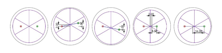
This is easier to see in Fig. 12 and 13 that summarize the decenter and height error cases. In Fig. 12 we look at a top view of the SMR, first, fully centered, then decentered 2 units up, then 2 units down. The 4th and 5th are decented 2 units left and right, respectively. In each case a line is drawn between the incident focus and the apex, and then continued on an equal distance beyond the apex to show the location of the reflected spot.

Fig. 12 Top view of SMR with incident (red) and reflected (green) spot positions as the cube corner is decentered within the ball

It is easy to see that a 2 unit decenter produces an 8 unit change in the reflected spot position upon a 180° rotation of the ball about an axis normal to Fig. 12. In reality, the motions in Fig. 12 are grossly exaggerated to show that effects of decenter. In practice, the decenters are a few tens of μm or less in commercial SMRs but the behavior of the reflected spot is the same as is shown.

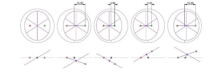
Fig. 13 is a diagram showing the situation for the apex being above or below the point of rotation looking from the top and side. We have shown how to calculate the distance above or below, but we need to know if the apex above or below the point of rotation for proper correction of the error. In the left hand view in Fig. 13 the SMR tips to the left but the apex (purple dot) lies on the center of rotation (black dot) so there is no motion of the apex and no displacement of the reflected spot (green). Also notice the distance between the incident spot and center of rotation is the same in all cases, only the reflected spot moves when the apex is not on the center of rotation.

Fig. 13. Top and side views where the apex is below and above the center of rotation when the SMR tips left or right.

In the second to left picture, the apex (purple dot) of the SMR lies below the axis of rotation (black) so the apex moves to the right as the SMR tips to the left, and vice versa in the middle picture. In fact, we do not tip left and right, but rotate the SMR 180° about the normal to the aperture of the cube corner, which has the same effect as tipping to the right. When the SMR rotates 180° the reflected spot moves to the left. If the apex is above the axis of rotation, as in the right hand two pictures, the reverse is true. Relative to the initial position of the reflected spot, the reflected spot moves right when the SMR is rotated 180°.

9. FIXTURE FOR MEASURING APEX LOCATION ERROR

Measuring the reflector apex location relative to the ball center requires two measurements of the reflected spot position with the reflector bisector vertical and two measurements while the reflector tilts as much as possible without vignetting, typically about 25°. With the reflector vertical, measure at an azimuth angle of 0 and 180°. Start the measurement as shown in Fig. 12, in the middle of one of the six pie shaped segments. This way the seam, or edge, of the segment does not block the beam by falling into the crack. The starting position is unimportant to the measurement because it only requires the difference in the two readings. However, if the cube corner needs centering, the direction of the decenter is important so the 0° reading should reference a feature on the SMR such as a logo or serial number.

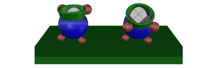
For the height measurement, the ball tilts about 25° and the spot position is measured. The ball is rotated 180° and the measurement repeated. Again, it is a difference measurement so the starting point is irrelevant. Even the precision of the 180° rotation is not critical because an error in this angle leads to a cosine error. Only gross errors in azimuth angle are significant. Fig. 14 shows a fixture that gives repeated proper orientation to typical SMRs.

Fig. 14. A fixture with the necessary features to perform apex location measurements. The Figure shows separate features for the two measurements required for clarity but the features easily combine into one fixture.

Three balls under the SMR locate the ball center precisely while two balls behind the collar (left) on the SMR hold the ball upright. The small black circles on the collar help orient the SMR during the 180° rotation. On the right, the two balls in front of the collar control the 25° tilt and the small circles help with the 180° rotation. The Figure shows the fixture as two fixtures for clarity but obviously, the two sets of two balls could combine into one fixture.

10. EXPERIMENTAL DATA

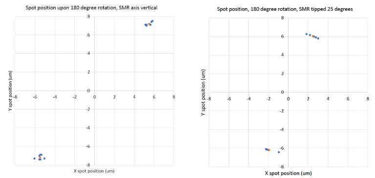
We tested a commercially available SMR sold as a standard quality SMR for reflector apex position using the methods outlined above. The standard quality designation means the apex lies within a sphere of radius 0.0005” (12.7 μm) of the center of the ball. Six measurements were made using the engraved logo as the azimuthal reference for 0 degrees and then at 180 degrees. The left chart in Fig. 15 shows the data with the orange spot being the average in the two locations. The x, y average coordinates were 5.50, 7.18 and -5.50, -7.18 μm for a spot separation of 18.09 μm at an angle of 52.6°. Since the sensitivity of the measurement is 4 times the spot separation due to the 180° rotation and doubling on reflection, the apex is 4.5 μm from the ball center at an angle of 142.6° relative to the serial number that was at the negative end of the y axis in the test setup. For decenter, this SMR meets the 0,0005” specification.

Fig. 15 Measured spot position data with the SMR vertical (left) and tipped the the right by 25° (right)

When we tipped the SMR -25° about the y axis, as opposed to Fig. 14 showing the fixture with the tip about the x axis, and repeated the measurement to get the data in the graph on the right. The average locations of the spots were 2.47, 6.01 and -1.93, -6.20 for a separation of 12.98 μm. Since the sensitivity of the measurement is increased by the sin of the angle of tip, the actual height difference between the apex and ball center is 12.98/(4*sin(25)) = 7.68 μm. Comparison of the two charts shows that when the SMR was tilted a -25° about the y axis, the x error became less indicating the apex is below the ball center. Notice the data in the y direction remains nearly the same whether the ball is tipped or not.

There are subtleties to the measurement that are not obvious at first. For one, the data shown are after subtracting the average reflected spot position because the actual distance of the incident light from the apex is completely arbitrary. What is significant is the difference between the 0° and 180 ° readings and their azimuthal angle relative to some azimuthal feature on the SMR. The arbitrariness is very useful in that it allows flexibility to avoid contamination on the corner reflector from affecting the measurement.

Also, the height and decenter measurements are coupled since tipping the SMR moves the apex laterally if the apex is above or below the ball center. This is why we measure the decenter with the reflector axis vertical, to avoid coupling in the height error. When the SMR tilts about, say, the x axis, the lateral positon of the x decenter does not change but the y decenter does if the apex is above or below the ball center. The direction of this change with tipping indicates whether the apex is high or low.

The advantages of the measurement method are clear. The test uses the simplest sort of fixture and the sensitivity of the measurement is well above the specification of the highest quality SMRs. Four data points are all that are needed to completely specify the location of the reflector apex relative to the center of the ball. It is easy to make the 4 measurements using the fixture and a suitable autostigmatic microscope in under 1 minute per SMR. Obviously repeated measurements should be made to assure a level of repeatability to meet quality assurance standards.

Since SMRs are used in many orientations, the risk of the SMR falling and being damaged is high. If the SMR is obviously broken there is only one solution; replace the SMR. On the other hand, the SMR may not show any sign of damage but the retro-reflector may have moved. This measurement technique is a quick check on possible damage.

11. CONCLUSION

We have shown how to measure the distance, in all three directions, of the apex of a spherically mounted retroreflector (SMR) relative to the center of the ball in which it is mounted. The measuring technique is simple, requires a simple fixture and is about 10 times as precise as industry standards.

12. ACKNOWLEDGEMENT

I would to acknowledge John Casstevens, of Dallas Optical Systems, Inc., for recognizing the possibility that the PSM might be applicable to measuring the location of the apex in an SMR, and for introducing the idea to Joe Gleason of Baltec, who subsequently stopped by to see if he could interest me into making the measurement. I would also like to acknowledge Robert Bridges of FARO Technologies, Inc. for providing SMRs to make additional measurements.

13. REFERENCES

[1] https://hubbsmachine.com/10-laser-tracker-875-sphere-mount-

[2] https://apisensor.com

[3] https://leica-geosystems.com/en-us/products/laser-tracker-systems

[4] https://www.faro.com/products/3d-manufacturing/faro-laser-tracker

[5] Steel, W. H., “The autostigmatic microscope”, Optics and Lasers in Engineering, 4, 217-27 (1983).

[6] https://www.optiper.com/products/point-source-microscope

Design For Alignment

Written by csadmin on June 27, 2019. Posted in Centering, Published Papers. No Comments on Design For Alignment

1. INTRODUCTION

The premise of this paper is that the only remaining way to improve optical system performance is with better alignment techniques. We feel optical design is a mature field and that little can be done to improve the design of optical systems by improvements to lens design software. The software may become easier or more convenient to use but the optical designs produced are near optimum given the design constraints specifying the system.

The same holds for the manufacture of optical elements. Between computer controlled manufacturing methods and interferometric testing of the manufactured elements and the many improvements in optical glass quality, not many avenues are open to improved quality of the optical components themselves. The only area left for improvement in performance of precision, or high quality, optical systems is the assembly and alignment of the glass elements and mirrors into mechanical cells, and lens benches, for more complex system geometries.

Based on this premise we will first define our concept of what precision optical alignment means and why traditional methods of alignment have not kept up with the improvements in lens design and the manufacture of high quality optical elements. We contrast traditional methods with more modern methods of optical alignment that make use of optical datums rather than mechanical datums and show the advantages of the optical methods.

Next, we show some advances in the optical methods of alignment including newer optical alignment tools and tooling including gratings that define axes in 5 degrees of freedom and how these make alignment easier. Finally, we look at the implications of these newer methods on how the opto-mechanics of cell and lens bench design are impacted so that tolerances can be loosened while achieving improved optical system performance. While this applies largely to precision optics manufacture, there are aspects of this approach that are applicable to production assembly as well.

2. MEANING OF OPTICAL ALIGNMENT

One might ask why is it even necessary to describe the meaning of alignment until you look in books and papers on optical design and manufacture for the words “alignment” or “centering” in their indices. The words are almost non- existent. This is why I think it is important to write about alignment because few people think about alignment until a kit of optical and mechanical components are set on a table in assembly area along with an assembly drawing. By then it is far too late in the process to make alignment any easier or more precise. Tolerances are assigned to the glass and metal parts in the design phase with the thought that if the parts are assembled per print, a system can be built that will perform as expected, but little thought is given to the process of putting the parts together to the tolerances given.

First, alignment is a paraxial concept based on the radii of curvature of surfaces, and the distances and the index of refraction between surfaces. The angles made a by misalignment are assumed small and the angles of rays through surfaces relative to normals of the surfaces are small enough that the small angle approximation sin α = α holds. This means that even if we want to align a large diameter surface we only have to look at a small region of the surface because we assume the surface is continuous with no abrupt changes.

The next concept is the difference between optical datums and mechanical datums to define alignment. The simplest of all optical surfaces is a spherical surface where we include plano surfaces as spheres with infinite radii, the same as do lens design programs. Optically, spherical surfaces are completely defined by 4 degrees of freedom; the location of the center of curvature and the radius of curvature as is obvious from the defining geometrical equation r^2 = x^2 + y^2 + z^2. However, when that infinitely thin spherical surface becomes physical by giving it some thickness it now has an edge that gives it a mechanical axis, but that axis has nothing to do with how the surface behaves optically.

The simplest way of showing this difference in optical and mechanical behavior is that there are two ways of moving the center of curvature to a particular location in space, either by displacement, or by tilting about the surface as shown in Fig. 1. If light is coming from infinity, or from near the center of curvature, the edge of the spherical surface will not affect how or where the surface focuses the light. At most, the edge will affect uniformity of illumination of the surface.

Fig. 1. Moving the center of curvature of a spherical surface by either displacement or tilt.

On the other hand, it pays to point out for future reference that if the location of the spherical surface is defined by a circular seat, it is not possible to move the center of curvature by sliding the surface in the seat. Sliding will move the physical edge of the (infinitely thin) surface but the center of curvature remains fixed in space because the intersection of a sphere cut by a plane is a circle.

Fig 2. Sliding a spherical surface sitting on a circular seat moves its edge but not its center of curvature.

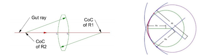
Finally, while a spherical surface does not have an optical axis, a lens with two spherical surfaces or an aspherical surface does have an optical axis. In the case of the lens, the optical axis is the line joining the two centers of curvature, period. The optical axis has nothing to do with the mechanical axis defined by the periphery of the lens. For an aspheric surface, the optical axis is defined the line between the vertex center of curvature and the sagittal center of curvature at the edge of the mirror aperture as in Fig. 3. For a parabola the length of that line is the same as the sag of the parabola, a short distance relative to the diameter unless it is a very fast parabola.

With these concepts in mind, the definition of alignment is to assemble the optical system so the centers of curvature and the optical axes of the components are precisely located as shown in the optical design model on the computer screen of the lens designer. This is simple to say but the actual task to accomplish this precise positioning of optical datums given a pile of discrete glass and metal components set out on an assembly workbench is difficult.

Fig. 3. Optical axis of a lens is line between centers of curvature, axis of asphere is line between the vertex center of curvature and the sagittal center of curvature at the edge of the mirror aperture.

3. TRADITIONAL APPROACHES TO OPTICAL ALIGNMENT

The traditional approach to optical assembly uses mechanical methods for several reasons. A mechanical designer did the mechanical drawings describing both the optical and mechanical components of the assembly. Assuming an incoming inspection was done on the components, mechanical rather than optical inspection was done because it is difficult to impossible to inspect individual lenses for optical quality outside an optical shop and even there it is difficult to do a functional transmission test. The people doing assembly tend to have greater familiarity with mechanical tools like micrometers, indicators and rotary tables than with optical tools like microscopes and alignment telescopes.

The traditional approach to centering lenses in a barrel or cell is to edge the lens to tight tolerances so the optical and mechanical axes are coincident when assembled. The cell is machined to tight tolerances to keep the seat centered and the bore just large enough so the edged lens will just fit. In this case there is no active centering, but reliance on tight tolerances to hold tilt and decenter of the lens to a minimum. However, there must always be a little gap between lens and bore or the lens would not fit in the bore. The tolerance stack up here limits the precision of centering and is costly because of the tight tolerances on both the glass and metal parts.

Another traditional method for perfect alignment, at least in theory, is using a precision rotary table and mechanical indicator. First, the seat is centered using the rotary table to establish a reference axis in space and an indicator to ensure the seat is concentric to the rotary table axis. As mentioned above, the seat will determine the location of the center of curvature of the spherical surface supported by the seat. Then the lens is placed on the seat, and the lens surface directly on the seat is slid on the seat until an indicator placed at the edge of the upper lens surface shows a constant reading. This shows there is a constant thickness of glass between the seat and the upper surface of the lens indicating coincidence of the optical axis of the lens and the rotary table axis, or that there is no wedge between the front and rear lens surfaces. Then the lens is constrained in the cell or barrel.

The positive aspects of the traditional method of centering is that it works, and has worked for many years. Another advantage is that since the elements are actively centered, the tolerances on edging the elements can be looser and the diameters of the bores looser. The seats must be precisely centered as there is no way of perfectly compensating for seat decenter by tilting the lens in the seat. In addition, the equipment used is familiar to most of the people doing the assembly.

Some disadvantages of the method are that it is a contact method and there is the possibility of the indicator tip scratching the lens. The lens being centered is often down inside a cell or barrel and it is sometimes difficult to get the indicator tip positioned on the edge of the lens, particularly with the indicator probe tip at an angle to get maximum sensitivity from the indicator. Further, precision rotary tables are expensive and require periodic maintenance for best performance.

Perhaps the most important shortcoming is that the datum of prime interest, the centers of curvature, are not accessed directly. Rather the position of the center of curvature is surmised from the touch indicator probe rather than measuring the location of the center of curvature directly as can be done optically. Unless the lens radii are very short, monitoring the lens edge is much less sensitive to alignment than viewing the motion of the center of curvature as the cell rotates.

4. NON-CONTACT METHODS OF CENTERING

Most non-contact methods of centering still require a precision rotary table but use an optical sensor to locate the center of curvature or its back focus of the element in question. Some systems also use a collimated beam of light coming up through the rotary table so the optical sensor above the lens can sense a transmitted focus. The sensors in these non-contact systems are autostigmatic microscopes^1,2 or their functional equivalent of an autocollimator with a focusing objective^3,4.

As centering proceeds, the focused spot viewed by the sensor precesses in synchronism with the rotary table, the magnitude of the precession getting smaller the better the centration. The focused spot stands still when the lens is perfectly centered on the rotary table axis. Among the advantages of this system of alignment is that the vertical column to which the sensor is mounted need not be perfectly aligned parallel to the rotary table axis nor does the column have to be perfectly straight. The indication of “perfect” alignment or centering is that the focused spot remains stationary as the table rotates even though the spot may not appear centered in the sensor’s field of view⁵.

The reference axis in space is the axis created by the rotary motion of the table and the axis extends without limit above and below the table. The focused spot from the lens conjugate is stationary only when the center of curvature, or back focus, lies on the axis created by the table rotation.

5. CENTERING WITHOUT A ROTARY TABLE

Recently we showed that Axicon gratings also create a reference axis in space without using a rotary table⁶ This allows non-contact centering while reducing the cost of the centering equipment and simplifying the centering itself. The grating method makes possible the viewing of 2 conjugates of a lens simultaneously, and thus the optical axis of a lens in one measurement. This way tilt and center are adjusted without any movement of the sensor or rotation of the lens being centered. There is immediate hand/eye feedback to the adjustments so the actual centering operation is simple and rapid.

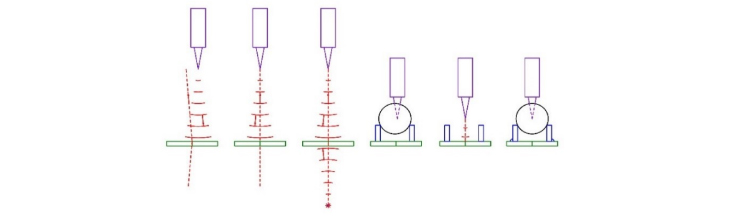
While the method of using an Axicon grating was described previously⁷, it is worthwhile illustrating again with a simple example of centering a doublet for cementing. Consider the steps in the Fig. 4 to set up the instrument for cementing.

Fig. 4. Steps to align the chuck, or seat, for cementing a doublet

The first picture shows an autostigmatic microscope (ASM) projecting a spherical wavefront from the focus of its objective toward the Axicon grating (green). When the spherical wavefront strikes the grating, diffraction produces two axial beams, one transmitted and one reflected (dotted red lines). The transmitted beam lies on the line joining the objective focus and the center of the Axicon grating pattern. The reflected beam is a mirror image of the transmitted beam.

As the ASM moves to the left in the next picture, the reflected beam appears as a spot on the ASM sensor and moves toward the centered crosshair in the ASM. When the focus of the ASM is on the axis of the grating pattern, the spot lies centered on the ASM crosshairs. With the ASM centered on the Axicon grating, a point source of light behind the grating (red dot) is adjusted laterally until the beam produced by the source is also centered on the crosshairs in the ASM. At this point both the ASM objective focus and the point source behind the grating lie on a line through the center of the Axicon grating pattern and normal to the grating pattern. Assuming a distance of 200 mm from the grating and an ASM sensitivity of 0.2 μm to centering the spot, the ASM and point source are aligned to the grating to 1 arc second.

In the fourth picture, we align the seat for cementing the meniscus half of the doublet to the grating using a spherical ball, for short radii, or the actual meniscus lens for longer radii. Note that the seat must be parallel to the grating as well as centered. The ASM is lowered on the vertical stage until its focus is at the center of the ball. Moving the ASM vertically will usually decenter the ASM from the center of the grating. This is why the ball is temporarily removed from the seat so the ASM can be re-aligned to the grating at this height. The ball is replaced after the ASM centering and the seat is centered so the reflected spot from the ball center is centered on the ASM crosshair with sub-micron precision. Now the seat, or chuck, is fixed in place relative to the grating and is not centered again. This completes the setup for cementing doublets.

Another approach to this setup step is to build the Axicon grating into the chuck so that it is pre-aligned to the grating in centering and tilt. There is no need for further alignment of the two unless there is damage to the lens seat that would disturb the alignment.

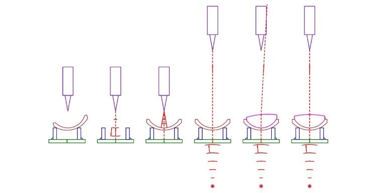
Fig. 5. Steps of aligning the two halves of the doublet for cementing

Fig. 5 first shows the ASM is adjusted vertically to be at the height of the center of curvature of the concave side of the meniscus. Moving the stage vertically will usually decenter the ASM slightly with respect to the grating. In the next picture, the ASM is centered on the grating after removing the lens to remove any misalignment.

Once the ASM is centered, the lens is replaced and slid on its convex surface on the seat until the center of curvature of the concave side lies on the axis of the grating as seen with the ASM. Since the center of curvature of the convex side is already on the axis of the grating because the seat is centered, the optical axis of the meniscus is coincident with the axis of the grating. The meniscus is fixed to the seat so it will not move during the cementing of the positive element. A convenient method of doing this is to use vacuum.

The ASM is moved up above the meniscus to a convenient height where it is out of the way of the cementing operation. The particular height is unimportant because the projected beam from below the grating is not affected by the power of the meniscus as will be shown below. Once the ASM is at a convenient height, the point source behind the grating is illuminated and used to center the ASM laterally. This is a precise centration of the ASM since the meniscus was well centered in both tilt and decenter. The transmitted beam from below the lens is incident on both meniscus lens surfaces at normal incidence so the beam is undeviated.

After placing a drop of cement on the concave surface, the positive element set on the meniscus. Since this element is not centered initially, the transmitted beam will be deviated until the element is centered. Once centered, after the cement is worked to the edge of the lens, the beam will be undeviated as shown in the last picture. The doublet is ready for curing of the cement.

6. INDEPENDENCE OF THE AXICON GRATING WITH LENS POWER

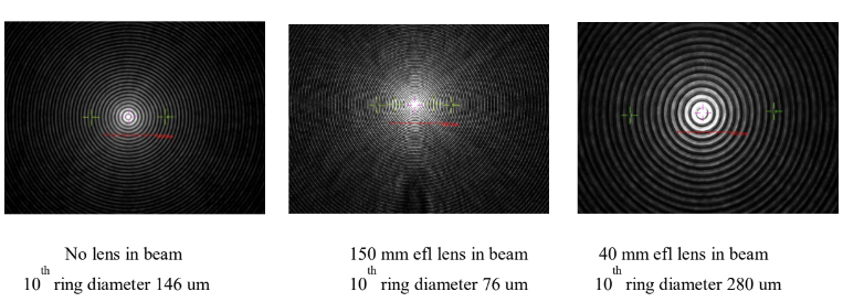
To demonstrate that the beam created by the grating is unaffected in its ability to center a lens independent of the power of the lens a couple of examples are shown in Fig.6.

Fig. 6. The spot produced by the transmitted beam through the Axicon grating and lenses of different powers as seen on the video screen of the Point Source Microscope (PSM), a commercial ASM

In the left hand picture of Fig. 6 there was no lens in the beam. In the middle picture, a 150 mm efl lens was inserted and centered. The centroiding algorithm still works just as well as in the left hand picture but the ring spacing is changed. Similarly, for the right hand picture where a 40 mm efl lens was inserted. The scale bar in red shows the same magnification for all 3 pictures and the green crosses were used to estimate the diameters of the 10th rings.

We point out that the reason the centroiding algorithm works in the Point Source Microscope (PSM)1 independent of the ring diameters is that the intensity of the brightest pixels is kept just under saturation when the Auto Gain function is used. Each ring of the spot pattern, including the central spot, has the same energy, but the intensity of the central spot is about 12 times that of the first ring surrounding it8. The centroid is calculated only using pixels within half the intensity of the brightest pixels and thus none of the light in even the first ring is included in the centroid calculation.

Before moving on to the design of hardware making use of these tools, we emphasize the power of these methods, particularly the use of the Axicon grating. The axis created by the grating defines 5 degrees of freedom, 3 translational and 2 angular. In one way, consider the grating a plane mirror with a defined axis strictly perpendicular to the grating surface that is easily located laterally to < 1 μm at almost any distance from the grating.

A further advantage of the Axicon grating is the ease with which the spot is aligned even when grossly misaligned to start with. Because the rings produced by the grating extend beyond the diameter of the grating, the curvature of the grating lines show which way the grating or ASM moves to achieve alignment. This is contrasted with using an autocollimator where most of your time is spent finding the return reflection. With the grating, unless you are vastly misaligned there is always a visible return reflection and that reflection indicates the way to move to achieve alignment of the spot.

No lens in beam 150 mm efl lens in beam 40 mm efl lens in beam 10th ring diameter 146 um 10th ring diameter 76 um 10th ring diameter 280 um

7. DESIGN OF LENS MOUNTING HARDWARE

As pointed out earlier, a spherical surface sitting on a circular seat will always have its center of curvature centered on the circular seat. This means that any lens with a second spherical surface can always be aligned so that the optical axis of the lens is coincident with the axis of the seat by sliding the lens in the seat, or at least until the edge of the lens interferes with the cell bore. The proviso here is that for multiple elements, the seats for the lenses must be concentric and that axis defined by the concentric seats must be aligned to either the axis of a rotary table or the axis of an Axicon grating before the property of tilting lenses is of any use.

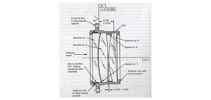
This situation calls to mind an illustration in Yoder’s book about opto-mechanical alignment shown below⁹. Here the primary datum is everyone’s wish, the cell and optical elements are all centered on this datum that is obviously the axis of both the elements and the cell. The problem is finding this axis using practical hardware, and is it an optical or a mechanical datum? It seems to me that much more practical datums would be the face of the cell as the A datum where it would sit on a surface plate or rotary table, and the B datum a bore in the cell. This gives a meaningful way of calling out other feature tolerances relative to easily accessible datum features rather than something that only is useful to the optical designer.

Fig. 7. Drawing of a lens assembly with an ambiguous primary datum (P. Yoder, Opto-Mechanical Systems Design)

Perhaps a fairer way of looking at Fig. 7 is to assume this is the assembled lens and the B datum should be perpendicular to A for mounting of the whole lens. However, the Figure is a great example of what to avoid when making mechanical drawings, datums that have little relevance to actual methods of inspection and assembly.

The text accompanying the Figure talks about the tight tolerances on the lenses and cell to achieve precision centering¹⁰. The tight tolerances mean expensive components and a difficult and risky job of assembly. Inserting close fitting elements into a tight bore call for a very steady hand. The least mis-alignment as the element is inserted in the cell will cause the element to jam against the bore. The element must never be forced, but gently backed out and inserted again. There is a high likelihood of chipping the element in this process.

Counter to this example, I would suggest the method used in microscope objective assemblies and that used for most lithographic lenses, cells, or bond rings, for each element going into an assembly as shown in Fig. 8 of this microscope objective. Notice every pair of elements is mounted in its own cell and, where possible, against a spherical surface. The design is complex enough that all details are not apparent in the picture but the concept is clear. By mounting each element is its own cell it is possible to align the optical axis of the element perpendicular to the face of the cell. Then as the individual cells are assembled, the only alignment is decenter and element to element spacing. This approach decouples tilt from decenter so the alignments are independent of each other.

Fig. 8. Cross section of a high power microscope objective

Another advantage with simpler systems than microscope objectives is you are not working down a bore but the lens vertices are largely co-planar with the faces of the individual cells. This makes it easy to measure lens vertex to cell face spacing and ultimately to correct element spacing during the centering step of assembly without having to worry about lens tilt. The method is largely self checking in that as cells are stacked up, the upper most cell face should be parallel to the bottom of the stack, and the thickness of the stack is easily measured via the cells rather than having to indicate off the lens vertices.

The idea of using bond rings, or individual cells, is not new. Yoder has several examples of this method of assembly and alignment¹¹. However, there is little emphasis on the advantages of this approach to assembly and alignment, some of which have already been mentioned. An even greater advantage than assembling lenses in a barrel comes with 2 or 3 dimensional optical layouts.

When lenses are assembled in a barrel, it is usually the case that gravity is working for you. In multi-dimensional cases, the system often cannot be orientated so that gravity aids the assembly. Decenter is not a big problem because it is easy to fixture a situation where 2 plane surfaces have to slide over each other to achieve alignment. Conversely, it is quite difficult to fixture an element that must rotate when it is not being held down by gravity. If an element can be mounted free of tilt in a plane cell with gravity aiding the alignment, and then centered against another plane surface where gravity is not helping, this is so much easier than fighting gravity where it is a tilt adjustment, or much worse fighting with tilt and decenter simultaneously.

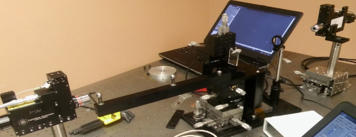
We use an example where a rectangular lens was edged out of a symmetric meniscus far enough off axis that the mechanical axis of the symmetric lens missed the rectangular aperture. The lens was then aligned to an “L” shaped mount in 5 degrees of freedom using a sophisticated fixture that allowed fine adjustment in the 5 degrees of freedom. We used two PSMs and an auxiliary lens to simultaneously locate both centers of curvature of the lens and guide the lens into position to be cemented. The alignment was quite easy but did required a fancy fixture with 7 precision stages. Fig. 9 shows the alignment setup.

Note the two tooling balls in Fig. 9 that locate the centers of curvature of the 2 sides of the rectangular lens (sitting in front of the upper laptop). Also, note the auxiliary lens next to the laptop that converges light onto the convex side of the lens. When the lens is not in the fixture light from the auxiliary lens focuses at the center of the tooling ball nearest the lens. The tooling balls are removed during the alignment of the lens so both lens surfaces are seen simultaneously.
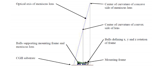
If instead the lens had been bonded in a cell that removed the tilt and then slid over a plane mounting surface machined into the lens bench at the correct angle relative to the other components the need for the complex fixture and dual ASMs would not be needed. Fig. 10 shows the same optical features as Fig. 9 with the 2 centers of curvature defining the optical axis of the lens and the rectangular lens hidden inside the lens mount (green). The lens and mount sit on a photomask substrate that has a set of Fresnel zone patterns defining the locations of precision steel balls that then kinematically define the locations of the lens and mounting frame^12,13. The layout of the photomask patterns is shown as a top view in Fig. 11.

Fig. 9 Setup for aligning a rectangular meniscus lens to a mount via a precision fixture

Fig. 10. Side view of a simple fixture to align the rectangular lens shown in Fig. 9

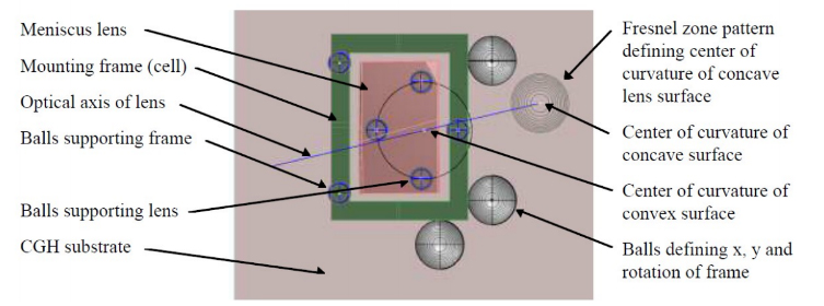
Fig. 11 Top view of the fixture used for alignment of the rectangular lens to is mount

Before describing the layout in Fig. 11 we should explain the use of the Fresnel zone rather than Axicon patterns on this photomask substrate. In the same manner as the equally spaced concentric rings of the Axicon grating, a pattern of Fresnel zone rings of varying spacings and widths are written on the substrate. By choosing the correct parameters, the Fresnel patterns will behave optically identically to concave spherical mirrors of a specific radius of curvature¹⁴.

By making the radii match the radii of steel balls, an ASM is first aligned to the center of curvature of the Fresnel pattern that is one radius above the substrate, and then a ball of that same radius is cemented to the substrate after being aligned to the ASM. Using this, technique the balls are aligned spatially to tolerances of about 1 μm in x and y. The Fresnel zone patterns typically have an overall spatial registration to the design location of 30-40 nm on a 150 mm square photomask substrate¹⁶.

In Fig. 11 the 3 balls under the pink rectangular lens define the location of the center of curvature of the convex surface of the lens in the same manner as a circular seat in the case of a symmetric lens¹⁵. The 3 balls under the green lens mount define the plane of the mount while the 3 balls at the edges of the mount define its x, y and z rotation. These 3 balls are unnecessary in theory because we will use these degrees of freedom to align the lens to the lens bench, but the mount must be held in place during cementing of the lens to the mount so these balls prove useful in a capacity other than alignment. In other situations, it is clear there is the possibility to completely define the location of the mount using the grating pattern and balls.

Prior to cementing the lens in the mount, an ASM is centered so the focus of its objective is at the center of curvature of the Fresnel zone pattern that defines the location of the center of curvature of the concave side of the lens. The lens is slid on the 3 balls until the reflected spot is centered on the ASM crosshairs, an indication that the optical axis of the lens is located correctly relative to the lens mount. Once cemented in its mount, the lens can be aligned to a plane surface in the lens bench by decenter alone by viewing a light beam produced by an Axicon grating. The mounted lens is slid on a plane surface of the lens bench machined at the correct angle until the Axicon beam shows no deviation with the lens in place.

Contrast of the 2 methods of alignment is stark. One photomask with a custom set of Fresnel zone patterns replaces one ASM, 9 or 10 precision stages and a sizable bit of real estate on an optical table. Further, in the actual cementing operation the method using the photomask is much easier ergonomically.

8. CONCLUSIONS

We have claimed that alignment is the only area where precision optical system performance can be improved and have attempted to show that traditional mechanical methods of improving alignment are difficult. Improvements to the precision of alignment and the ease of assembly are relatively easy to make if one thinks about alignment in the design phase of the system and applies optical rather than mechanical methods of alignment.

9. ACKNOWLEDGEMENT

The author acknowledges the help of Dr. Chenyu Zhao of Arizona Optical Metrology for providing prototype Axicon and Fresnel zone gratings.

10. REFERENCES

[1] https://optiper.com/products/point-source-microscope
[2] https://opt-e.com/wp-content/uploads/2016/02/Opt-E-W2-2016-02-13-1.pdf
[3] https://trioptics-usa.com/products/opticentric
[4] https://www.optoalignment.com/las-bt-vis
[5] Parks, R. E., “Practical alignment using an autostigmatic microscope”, Proc. SPIE 8491, 84910H (2012).
[6] Parks, R. E., “Alignment using Axicon plane gratings”, Proc. SPIE 10747, 1074703 (2018).
[7] Parks, R. E., “New approach to optical assembly and cementing”, Proc. SPIE 10747, 107470C (2018).
[8] Liu, X. and Xue, C., “Intensity distribution of diffractive axicon with the optical angular spectrum theory”, Optik 163, 91-8 (2018).
[9] Yoder, P., [Opto-Mechanical Systems Design, 3rd ed.], CRC Press, Boca Raton, FL, p. 238 (2006).
[10] Ibid.
[11] Yoder, op. cit., pp. 285-97.
[12] Coyle, L., Dubin, M. and Burge, J., “Low uncertainty alignment procedure using computer generated holograms”, Proc. SPIE 8131, 81310B (2011).
[13] Parks, R. E., “Optical alignment using a CGH and an autostigmatic microscope”, Proc. SPIE 10377, 1037703 (2017).
[14] Coyle, op. cit.
[15] Parks, R. E., “Computer generated holograms as fixtures for testing optical elements”, Optical Design and Fabrication 2017 (Freeform, IODC, OFT), OSA Technical Digest (online) (Optical Society of America, 2017), paper JTh4B.4.
[16] Ekberg, P. and von Sydow, A., “Past and future challenges from a display mask writer perspective”, Proc. SPIE, 8441, 84410N (2012).

Videos From the Optical Society

Written by csadmin on September 21, 2018. Posted in News. No Comments on Videos From the Optical Society

OSA Stories

The Optical Society offered Robert (Bob) Parks an opportunity to share his stories of excitement and inspiration in a couple of short videos.

(ANNOUNCEMENT FROM THE OPTICAL SOCIETY)

OSA CAM VIDEOS

We’re Celebrating All Members (CAM) by inviting members attending many OSA meetings and congresses with an opportunity to share their stories.

View OSA Stories videos on Optiper videos page here.

News Announcement About What is Happening in 2018 for OPG

Written by csadmin on May 19, 2018. Posted in News. No Comments on News Announcement About What is Happening in 2018 for OPG

For the last three years Optical Perspectives Group, LLC (OPG) had a licensing agreement with Trioptics-USA to manufacture and sell OPG products exclusively world-wide.

OPTICAL PERSPECTIVES GROUP, LLC (OPG) AND TRIOPTICS-USA MUTUALLY DECIDE TO END LICENSING AGREEMENT

Toward the end of last year it was becoming clear that this arrangement was not in the best interest of either group because we were selling our products into different markets.

We mutually decided to end the agreement as of December 31, 2017.

FROM NOW ON OPTICAL PERSPECTIVES WILL MANUFACTURE AND SELL OPG PRODUCTS WORLD-WIDE DIRECTLY AND THROUGH ITS OWN NETWORK OF INDEPENDENT SALES PEOPLE.

OPG feels this is the best way to support our customer base and to provide applications support for our products.

EXCITING NEW WAYS TO USE PSM WITH CUSTOM CGH

We are particularly excited about using the Point Source Microscope (PSM) along with custom Computer Generated Holograms (CGH) for the precision alignment of optical systems and the calibration of machine tools and automation equipment.

MORE INFORMATION ABOUT OPG PRODUCTS AND THEIR APPLICATIONS

Centering Steep Aspheric Surfaces

Written by csadmin on August 26, 2017. Posted in Centering, PSM Applications, Published Papers. No Comments on Centering Steep Aspheric Surfaces

1. INTRODUCTION

Finding the optical axis of an aspheric surface is an essential part of making an aspheric lens because the center of curvature, or optical axis, of the second side must lie on, or be coincident with, respectively, the optical axis of the first side for maximum optical performance. Looking at the center of an aspheric surface and measuring the tilt and coma as a function of decenter is an obvious means of determining centration, but many aspheric surfaces are relatively spherical over the part of the lens aperture that can be viewed with commercially available optics and there is too little coma to make a useful measurement of decenter.

We describe an alternative method of viewing a small patch of the aspheric surface near the edge of the clear aperture where the asphericity is greatest while rotating the lens about an axis close to coincident with the optical axis of the surface. By also tracking the reflected light image when using an autostigmatic microscope (ASM), or using an interferometer to measure the low order Zernike coefficients, as the lens is rotated, both the tilt and decenter of the surface can be determined.

The relationship between the image motion and Zernike coefficients is described for both tilt and decenter of the surface as well as the means of separating the relative amounts of tilt and decenter are given. These methods of determining tilt and decenter seem to work for all aspheric surfaces we have tried to date.

We begin by reviewing the thinking that led to the method described for finding the optical axis of an aspheric surface. The discussion moves through successive attempts to find a method of locating the optical axis for aspheric surfaces that works for all surfaces that have enough asphericity to qualify as aspheres. Results are shown for both the interferometer and the autostigmatic microscope method*. Finally, we conclude by describing a method that may work even better for many aspheric lenses that makes use of a computer generated hologram.

*After submitting the Abstract for this talk it came to the author’s attention that there is a European Patent #EP 1918 787 A1 covering the autostigmatic microscope method described in this paper for locating the optical axis of the first surface of an aspheric lens.

2. BACKGROUND

In the process of manufacturing precision aspheric lenses and surfaces, particularly lenses molded of glass, plastic or other optically useful materials, it is imperative to know if the optical axes of the surfaces are coincident for the best optical performance of the lens. There must be neither tilt or decenter between the optical axes. This requires a method of measuring the axes of both aspheric surfaces relative to each other, or relative to a common reference.

One method in wide use is a Panasonic UA3P coordinate measuring machine that measures relative to a common reference by mounting the lens in a plate with a hole the diameter of the lens so the lens surfaces can be reached from either side of the plate. The plate also has 3 balls mounted so they protrude from either side of the plate. The plate mounts against “V” grooves so that the plate may be turned over without the axis of the plate being lost. This is how both sides of a lens are measured relative to a common axis.

Although the UA3P is widely used it has limitations; it measures by contacting the sample with a probe tip which may damage soft lens materials such as plastics. Even for small lenses the measurement time is long, and while very precise, the machine is very expensive.

Another way of measuring the optical axes relative to each other is to mount the lens centered on a post that is centered on a rotary table. As long as one can access the edges of the optical surfaces they can be measured relative to the common axis of the rotary table¹. Again it is a contact method and is not very useful for small lenses such as might be used in cell phones and endoscopes. Further, it cannot fully determine the difference between tilt and decenter of the optical axis because while this method measures out at the edge of an aspheric surface where it is most sensitive to measure for tilt and decenter of the axis, measuring only displacement and not simultaneously tilt leaves some ambiguity in the definition of the axis of the surface.

A further method is disclosed in US Patent Application 2010/0309458, “Asphere Measurement Method and Apparatus”, where two interferometers are used facing each other with the lens being measured in between the two. This method is non-contact and purports to determine the optical axes of the two surfaces by measurement of the profiles of the two surfaces. In practice this method works well for some lens designs but probes the lenses in the centers of their surfaces, the place on the surface of some lenses least sensitive to the determination of the optical axis. The method of aligning the two interferometers to each other is vague in the patent application, yet this alignment is vitally important for a precise measurement. Finally the method requires two complete interferometers.

3. METHOD USING THE CENTER AND EDGE OF THE SURFACE

3.1 Using an interferometer

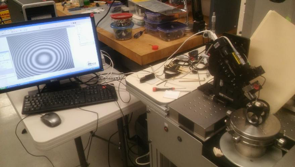
One method of looking at both the center and edge of an asphere is to use two interferometers equipped with Mirau objectives that compare the aspheric surface to a plane reference. This is a practical method of looking at the surfaces because the Mirau objective is the interferometer, and thus the entire interferometer package can be kept quite small. This makes it convenient to mount an interferometer so that it can look at a portion of a surface near the edge of the aperture as shown in Fig. 1 where the whole interferometer package is a Point Source Microscope² (PSM) and PZT phase shifter to move the Mirau objective.

Fig. 1 A PSM based Mirau interferometer viewing near the edge of an aspheric lens sitting on a rotary table

As seen on the monitor the fringes from the interferometer show astigmatism that is not centered in the field of view. The low order Zernike coefficients in each interferogram will change as the lens is rotated on the rotary table unless the lens is well centered. By using Zernike coefficients from an interferometer and those from viewing at the edge of the aperture the tilt and decenter of the surface can be separated and measured. While this method works well, and provides high precision it is instructive to look at using an ASM to do the same measurement because the ASM is a less expensive solution and easier to implement. The ASM explanation also gives some insight into what the interferograms and Zernike coefficients show about the centering. Further, the ASM method has some advantages when trying to center the second surface of the asphere over the interferometric approach.

3.2 Using an autostigmatic microscope

Using an ASM to determine the optical axis of an aspheric surface goes back to fundamentals. An axis is a line and a line is determined by 2 points on the line, or a point and an angle. The line in this case is the line between the paraxial center of curvature (CoC) of the surface and the sagittal focus, the point defined by the normal to the surface at the edge of the clear aperture of the lens. To illustrate the concept and keep the math relatively simple a parabolic surface will be used as the example.

3.2.1 Centering geometry illustrated using a convex parabola

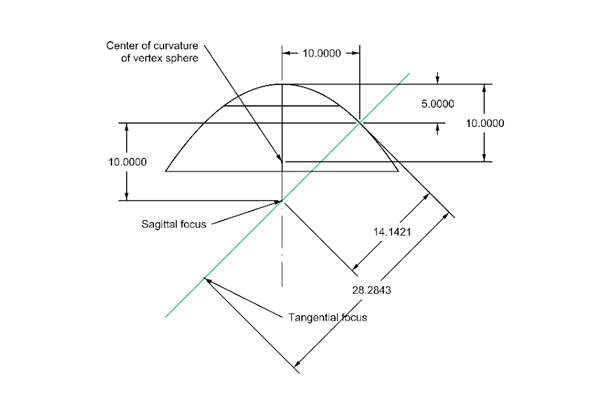
Consider a parabola with a 10 mm vertex radius large enough in diameter so that we can look at an annulus where the slope of the surface is 45°. Such a parabola is shown in Fig. 2 with relevant dimensions.

Fig. 2 Convex parabola with 10 mm vertex radius and zone at 10 mm radius

Before getting into the details of the dimensions in Fig. 2, it is important to understand the fundamentals of the problem of locating the optical axis of the aspheric surface. With an autostigmatic microscope (ASM) looking down in z along the optical axis and focused on the vertex radius of curvature, the position of the vertex CoC is monitored as the surface is rotated in azimuth about the z axis. The vertex CoC is one point on the optical axis and it is easy to get data in x and y on the ASM monitor as the surface rotates in azimuth, θ.

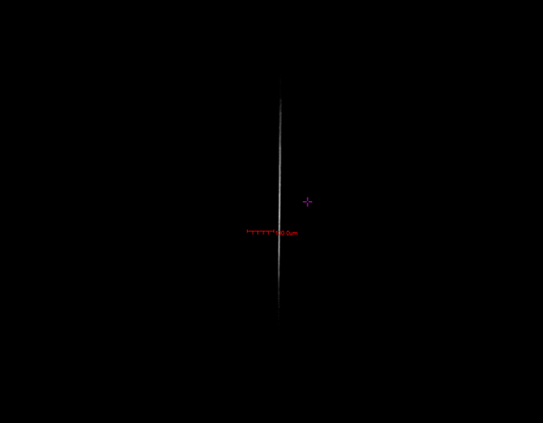
By looking normal to the surface toward the optical axis along a line 45° from the optical axis, the other point seen with an ASM is the sagittal focus, a second point on the optical axis. Since the sagittal focus is a line image in the plane of Fig. 2, it is ambiguous to measure the position of the line in a direction along the line image. However, it is easy to measure the displacement of the line perpendicular to the line. Fig. 3 shows a typical line image from the sagittal focus and it is clear that it is easy to determine the position of the line left to right, or in the x direction perpendicular to the line.

At first it seems the x location is insufficient information to determine the y position, but since the surface is rotating in θ, the y position of the line image will be 90° out of phase with the x position. This being the case, the two points on the line a known distance apart are completely defined, sufficient information to explicitly determine the optical axis of the surface relative to the axis of rotation of the rotary table.

Fig. 3 Image of the sagittal focus of an Edmund Optics asphere 69-141

This information also gives a means of calculating the sensitivity of the measurement based on the distance between the CoC of the vertex sphere and the sagittal focus. Clearly the angle of incidence of the beam focused at the sagittal focus should be chosen to maximize the distance between the CoC and the sagittal focus, usually a point at the edge of the clear aperture.

Another aspect of this geometry is that if the surface is moved relative to the axis of rotation so that there is no motion of the CoC, the surface is perfectly centered, that is, there is no decenter. If there is still motion of the sagittal image it is entirely due to tilt. This makes it easy to separate decenter of the surface from tilt, and makes the adjustment to eliminate tilt and decenter quite easy.

This geometry also sets up the possibility of measuring the relative tilt and decenter of the second surface of a lens by looking through the first surface. If there is no tilt or decenter of the first surface, there will be no motion of the reflected spots from the second surface introduced by the first. There will clearly be dependencies on the setup of the ASMs to measure the second surface that depend on the first, but once the first surface is centered and the initial setup is done, the first surface will not influence the second surface measurements as a function of θ.

3.2.2 Calculation of the dimensions of the relevant features of the parabola

Referring back to Fig. 2, the zone where the slope is 45° is 10 mm from the optical axis because y/R = 10/10 = 1 = tan(45°). The sag at y = 10 is y²/2R = 5 mm. The center of curvature of the vertex sphere is 10 mm below the vertex and the sagittal focus is sag + vertex radius = 5 + 10 = 15 mm below the vertex where the normal to the surface intersects the optical axis. The distance from the surface to the optical axis is sqrt(y² + R_v²) = sqrt(20) = 14.1421 mm, the sagittal radius, R_s. The distance from the surface to the tangential focus is R_t= R_s³/R_v² = 28.2843 mm, in this particular case of a parabola, 2*R_s.

If a converging beam of light from the ASM is directed normal to the surface at the zone y = 10 and is focused at the sagittal focus, the reflected light will form an image that is in the plane of Fig. 2 and perpendicular to the incident beam. This is because the sagittal focus is the center of curvature of the surface perpendicular to the Fig. 2.

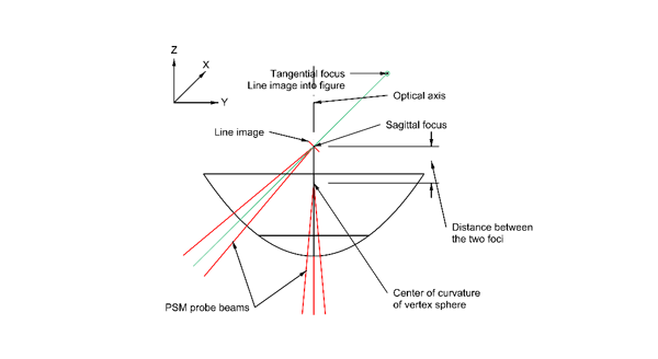
If that same beam is focused at the tangential focus, the line image formed by the reflected light will be perpendicular to Fig. 2. This is because the tangential focus is the center of curvature of the surface in the plane of Fig. 2. If one were to draw a circle whose center was the tangential focus and radius was R_t, the circle would be precisely tangent to the parabola at y = 10. Fig. 4 shows the geometry of the parabola and ASM probe beams before rotating the model.

This rather simple model was used as an aid in setting up a Zemax file to analyze more general examples of probing the sagittal foci aspheric surfaces. In Zemax, it is easiest to have the light coming in through a paraxial ASM from the left impinging on the surface at normal incidence. This means rotating the surface about the sagittal focus to accomplish this. The simple parabola model made it easy to see that the Lens Data file was set up correctly for more complex cases.

Fig. 4 Parabola model with PSM probe beams before 45 ° rotation

3.2.3 Example of investigating a general aspheric surface

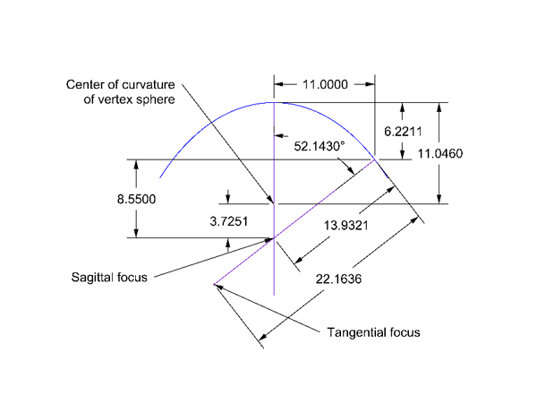
Edmund Optics sells a molded plano-convex aspheric lens (P/N 69-141) of similar dimensions to the parabolic surface just used as an example. The pertinent dimensions are shown in Fig. 5 and were derived from the information that Edmund² makes available on line or via the Zemax lens files. In the case of this lens a convenient tilt to probe the sagittal focus without vignetting the beam at the edge of the clear aperture is about 52°. This gives a separation of the CoC from the sagittal focus of 3.73 mm, a number that gives the sensitivity of the determination of the optical axis.

Fig. 5 Pertinent dimensions of Edmund aspheric lens 69-141 for determining the optical axis

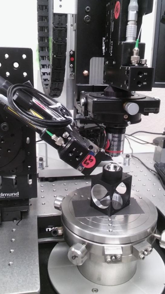
This lens was set up on a precision, air bearing, rotary table so that it could be viewed by two PSM’s, one looking down on axis and the other looking along a normal at 52° from the axis of the table. The setup is shown in Fig. 6.

The PSM on the left that is viewing the sagittal focus does not appear to have an objective, but it does have a 50 mm efl doublet used as an objective to give sufficient working distance so the two objectives do not interfere when making simultaneous measurements.

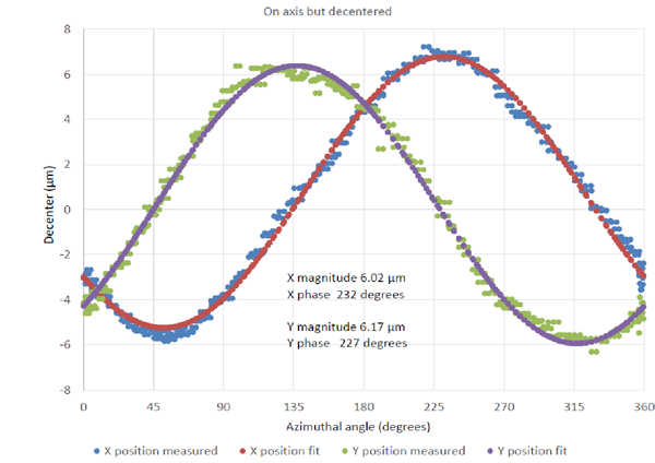
The first measurement done was to check the centering of the CoC of the vertex sphere with the PSM looking down the axis of the asphere. Fig. 7 shows the data from this measurement where data was taken for about 2.5 complete revolutions of the rotary table. The measurement data were continuous scans of the x and y reflected image positions from the CoC versus the table rotation axis. By taking multiple rotations it gives a feel for the repeatability of the data. To begin, the lens was reasonably well centered but, as the data shows, not to the level of sensitivity of the PSM.

Fig. 6 Edmund 69-141 lens on a rotary table being viewed by two PSM’s

Fig. 7 Measurement of the centering of the CoC of the Edmund lens before adjusting the centering

This data set is instructive from several viewpoints. First, the repeatability revolution to revolution is at the sub-micron level. When the data were least squares fit with sin curves the magnitudes and phases should have been identical if there were no measurement error. In fact the relative error in magnitude was about 2.5% and the relative phase error about 1.4%, rather good considering a centering error of about 6 μm. Further, the data indicates the azimuthal orientation of the centering error so that it can be corrected.

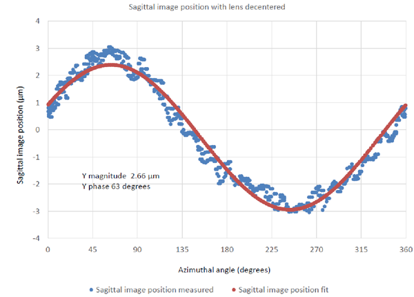
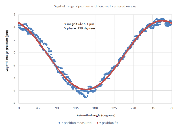
Before centering the lens the error at the sagittal focus was measured and is shown in Fig. 8. Here only the x direction data is shown as explained previously because of the line image. Again the repeatability for multiple rotations is sub-micron and very sinusoidal.

Fig. 8 Measurement of the centering error of the sagittal focus

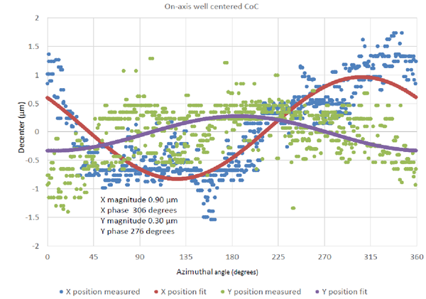
The lens was then translated to center the CoC as well as could be done given the limits of hardware and software. Fig. 9 shows the residual centering error of the CoC which is about 0.3 μm when the x and y data are averaged and it is recalled that the graph shows the total runout, twice the actual decenter from the rotary table axis.

Fig. 9 Residual centering error after best attempt at centering the CoC of the vertex sphere

Following the centering of the CoC the sagittal focus was re-measured without making any further adjustments, and this result is shown in Fig. 10. The magnitude of the error is slightly greater than before centering and the phase about 84°. This means the tilt of the optical axis is about 1.3 mradians relative to the rotary table axis.

Fig. 10 Centering error in the sagittal focus after center the CoC

3.3 Centering both sides of the plano-convex lens simultaneously

Since the lens in the example has a plano backside it is also possible the determine the tilt of the plano side relative to the rotary table axis by moving the on-axis PSM to the back focus of the lens as shown in Fig. 11 where the optics of the PSM are modelled as paraxial lenses.

Fig. 11 Rays from the PSM on-axis at the back focus of the Edmund lens

The back focus is 18.75 mm above the lens while the objective is focused 11.046 mm below the surface to focus at the CoC for a total focus shift of about 29.80 mm. In this back focus position, Fig. 12 shows the decenter of the spot from rays reflected off the plano surface. These curves look very similar to all the previous centering data with the exception that the decenter is larger and the two curves do not appear to be centered evenly about zero decenter. The even decenter about zero simply has to do with where the center of the reference in the ASM was set at the beginning of the measurement, and has no bearing on the data other than aesthetics. The fact that the decenter magnitude is much larger has to do with the much longer baseline over which the decenter is measured.

This data was taken when the CoC was centered as best we could and the CoC is 29.80 mm from the back focus. Thus the tilt of the plano surface is 53.3 μm/2*29800 μm = 0.89 mradians at an azimuthal angle of 252.5°, close to the angle of the optical axis relative to the rotary table. It appears that this lens is quite free of tilt between the aspheric surface and the plano side. The long distance between the two foci on axis gives a high sensitivity to this measurement of wedge in the lens.

Fig. 12 Decenter of the back focus of the lens

Because it was now obvious that 3 measurements could be made on the plano-convex asphere without moving the lens from its original fixture, it was decided to see if tilting and decentering the element could bring the optical axis of the whole element in line with the axis of the rotary table. By alternately focusing first at the CoC and then the back focus it was possible to center both conjugates to less than 1 μm. Given the nearly 30 mm distance between conjugates this means the error between the optical axis and the rotary table axis were no more than about 7 arc seconds. With this degree of alignment, another measurement was made of the centering error at the sagittal focus as shown in Fig. 13.

Fig. 13 Residual decenter of the sagittal focus after alignment of the back and CoC foci

This alignment of both sides of the shows the alignment can be done to high precision without having to turn the lens over to center the second side. We will go on to show that this works in the cases of both a spherical surface on the second side and an aspheric surface. By aligning both sides of a lens in one set up it eliminates the possibility of introducing mechanical misalignments in the process of turning the lens over so the second side can be measured. In this approach the only necessary condition is to align the first surface as well as possible to the axis of the rotary table so that when looking through the first surface the error in the alignment of that surface does not affect the measurements of the second side.

The only regret in this whole exercise was that it was not possible to get a mechanical indicator in the set up to measure the runout of the periphery of the lens. This would have shown whether the periphery could have been relied on to center this otherwise very good lens in terms of centering.

3.4 Measuring the alignment of two aspheric surfaces on a single lens in one setup

It is difficult to find a design of a lens with an asphere on both sides because of proprietary design issues but it is easy to illustrate using this method of alignment by going back to a lens with parabolic surfaces on both sides. The example is general and the explanation is simple because of the simple nature of the surfaces. Start with the parabolic surface shown in Fig. 1 and add to it a second positive parabolic surface with a vertex radius of 20 mm and a central thickness of 14 mm. Assume the element is 25 mm in diameter and made of a glass of index 1.6 to produce a lens the looks like Fig. 14 (a).

Fig. 14 (a) Double side parabolic aspheric lens (b) PSM at optical CoC of side 1

Assume the lens is sitting on a rotary table and side 1 has been centered in tilt and decenter relative to the rotary table axis as well as possible. The PSM that is on axis is used to look at the optical CoC of side 2 to determine whether that CoC is decentered. That configuration looks like Fig. 14 (b) where much of the PSM optics have been left out in order to better see the rays in the lens. If side 2 of the lens is decentered the index of the glass increases the sensitivity to decenter by the index, so a decenter of 1 μm leads to a TIR spot motion of 3.2 μ in this case of the 1.6 index. The index does not affect the apparent sensitivity to tilt because although it is affected, the greater sensitivity is reciprocally cancelled because of the apparent shorter lever arm the tilt acts over. However, by just looking on axis we cannot tell whether the motion in the reflected spot is due to decenter of the CoC or a tilt of side 2.

To check on side 2 to separate tilt from decenter there are an infinite number of solutions but introducing the PSM probe beam at an arbitrary angle as shown in Fig. 15, the light is reflected off the local CoC of a patch of the surface of side 2. Fig. 15 is complex but matches the Zemax model of this same situation exactly. The vertex of the lens was at 0,0 to begin with. It was arbitrarily decentered -3 mm and then tilted 26° about a point 3.994 mm beyond where the vertex was originally. Once this was done it is not hard to show the angle of incidence is 34.194° which makes the angle of refraction 20.563° where we use an index of 1.6. Fig. 16 (a) shows the Zemax layout of the model lens in Fig. 14 and Fig. 16 (b) shows the tangential image which is diffraction limited in the narrow direction.

Fig. 15 Double parabolic lens tilted and decentered so incident ray reflects normally at side 2

Fig. 16 (a) Zemax model showing the ray bundle reflecting off side 2 and (b) the tangential image seen in the PSM

By changing the merit function in Zemax to find the sagittal image, the thickness on surface 1 changes by 0.704 mm and the line image is vertical. The focus shift of 0.704 mm is all that is needed to go from one diffraction limited focus to the other on side 2. Either image could be used to check the centering of the second side.

It should be noted that the default Zemax merit functions that use the operands TRCX and TRCY to find Spot X or Spot Y. These operands do not work to find sagittal and tangential images. Use these default merit functions to get the pupil coordinates but change the operand from TRCX to REAX, or TRCY to REAY and enter the last surface as the place for the ray heights to be zero. This does a good job of finding the appropriate thicknesses and radii for the sagittal and tangential foci.

To conclude this aspect of the discussion it has been shown that using an ASM in two positions relative to an aspheric surface it is possible to unambiguously determine the location of the optical axis of the surface relative to the axis of a precision rotary table. Furthermore, once the first surface of the aspheric lens has been centered as well as possible to the rotary table axis, the ASM viewing the aspheric surface near its edge can be repositioned to obtain a reflection off the second surface sagittal or tangential center of curvature. Using this ASM and the ASM that is on axis but now focused at the second surface apparent center of curvature, it is possible to determine the tilt and decenter of the second aspheric surface without ever having to move the lens from its initial fixture on the rotary table. This single setup to measure the optical axis location of both surfaces leads to a more precise measurement than one where the lens must be flipped over to measure the second surface.

Computer Generated Holograms As Fixtures For Testing Optical Elements

Written by csadmin on July 19, 2017. Posted in PSM Applications, Published Papers. No Comments on Computer Generated Holograms As Fixtures For Testing Optical Elements

1. INTRODUCTION

It is common to think of computer generated holograms (CGH) as artifacts for testing aspheres but they can also be used as general calibration artifacts and fixtures for the alignment and test other more conventional optics. We show how simple Fresnel zone patterns can be created to simulate centers of curvature or axes in space with dimensional precision associated with microlithography. These centers of curvature and axes can then be located in space to similar sorts of precision with an autostigmatic microscope (ASM) or an interferometer.

Once the ASM is centered on the center of curvature, or axis, of the Fresnal zone pattern, a ball, or cylinder, respectively, of matching radius can be aligned to the ASM or interferometer to similar sorts of precision and physically attached to the CGH to serve as kinematic datums against or on which to mount other optical or mechanical components.

We then give an example of the fixture for the mounting of a rectangular lens element into a kinematically located frame so the two can be cemented together prior to inserting the bonded pair into an optical bench.

2. ORIGIN OF THE CONCEPT

From their earliest use as null devices for testing aspheres, CGH’s had to be precisely aligned to the interferometer used for the testing. This was originally done by attaching balls to the corners of the CGH’s using the mechanical features of the CGH’s as datums. More recently, Coyle [1] showed that the balls used for alignment could be attached to the CGH in a more precise way, and more importantly, one that was directly related to the aspheric test pattern by including in the overall CGH pattern, Fresnel zone patterns that defined the locations of the centers of the alignment balls.

While Coyle originated the idea of locating datum balls on CGH’s, she used a purpose built autocollimator with a monochromatic light source. The balls can be located just as easily and precisely with a commercially available ASM, or with an interferometer for even higher precision.

3. SECURE MOUNTING OF THE BALLS

In the original implementation of adding datum balls to CGH’s they were cemented directly to the CGH. The actual mechanical connection of a steel ball to a glass plate with an adhesive such as epoxy is problematic in two respects; the joint with the ball standing proud of the plate is highly susceptible to a lateral blow, and if the blow is sufficient to knock the ball loose there is a high likelihood of the cement pulling out a piece of the glass due to the nature of the bond.

We feel a better means of fastening the balls to the CGH is via the nests used for the SMR’s used in conjunction with laser trackers. The Fresnel zone pattern is adjusted in radius to compensate for the thickness of the nest and the ball/nest pair is used to locate the nest which is then cemented around it periphery. The lower profile of the nest makes it less vulnerable to getting a sideward blow and the greater area of the cemented joint makes it less likely the nest will be knocked off the CGH. Of course, in the worst in instance of the bond being broken the damage to the CGH would probably be greater.

4. EXAMPLE OF A FIXTURE FOR MOUNTING AN “OFF-AXIS” LENS

In this example it was required to align a rectangular meniscus lens element to its kinematically located mount so the two could be cemented together. The rectangular lens was cut out of the meniscus so the optical axis of the lens lay outside the lens as shown in the Fig. 1.The mount was designed with pins so that once the lens was aligned and cemented to the mount, the cemented pair could be deterministically located on an optical bench via the pins.

A CGH is laid out with a Fresnel zone pattern to focus light at the center of curvature of the concave side of the meniscus with allowance for the lens thickness and diameter of the balls. In addition, three balls are positioned relative to the Fresnel pattern to locate the center of curvature of the convex side to define the other end of the optical axis of the lens. When the lens is placed on the three balls, the center of curvature of the convex side will lie on the optical axis of the lens as defined by the position Fresnel pattern on the CGH and the center of curvature of the concave side it creates.

When an ASM is focused on the center of curvature of the concave side produced by the pattern, the lens is slid on the 3 balls until its center of curvature is centered in the ASM aligning the lens to the fixture. A metal fixture plate drilled to accept the pins on the mount is located on the CGH by 6 additional balls, 3 to determine a plane parallel to the CGH and of the correct height. Three other balls locate the plate in 2 degrees of translational freedom and one of rotation so that when the lens mount is mated with the plate, the mount is in the correct position relative to the lens as shown in Fig. 2. From a drawing of the plate and mount, Fresnel patterns are printed on the CGH for the 6 balls locating the fixture plate. Obviously the entire pattern is printed on the CGH at one time with the locations of the Fresnel patterns located to microlithographic precision.

5. OTHER ASPECTS OF CGH FIXTURES

Two other properties of the CGH’s used as fixtures should be mentioned. The first, pointed out by Coyle is that at each Fresnel location, centers of curvature are created on each side of the CGH so that these two centers of curvature establish an axis without having to autocollimate off the CGH, if this is useful during alignment. The other thing is that a pattern of equally spaced rings can be used to create an axis perpendicular to both sides of the CGH that extends indefinitely provided there is sufficient intensity in the focused point source of the ASM used to locate the axis. The equally spaced rings create an axicon that in turn creates a conical wavefront. The only disadvantage of this use of the CGH is that the efficiency of the pattern decreases with distance and the intensity of the point source must be increased with distance.

6. CONCLUSION

We have given an example of how a CGH may be used as a fixture for the alignment of optical and mechanical components when used in conjunction with an ASM to interrogate the CGH. We believe we have explained the method in sufficient detail that many other examples can be readily imagined. As another example, entire symmetric optical systems can be precisely aligned without the need for a rotary table; the axicon CGH creates the reference axis in space.

7. REFERENCES

[1] L. Coyle, “Precision Alignment and Calibration of Optical Systems Using Computer Generated Holograms”, Ph.D. dissertation, Univ. of Arizona (2014), https://hdl.handle.net/10150/332847.

Fig. 1 Menicus lens showing the “off-axis” rectangular lenses positioned relative to the axis of symmetry of the meniscus.

Fig. 2 CGH as a fixture for alignment of a rectangular lens relative to a mount designed to be pinned to an optical bench

Author: csadmin

Prism Alignment Using A Point Source Microscope

1. INTRODUCTION

2. USING SMRS

3. PRECISE POSITIONING OF LASER TRACKER NESTS

4. ORIGIN OF THE IDEA OF USING THE PSM TO MEASURE SMRS

5. IMAGING ON A SURFACE WITH A POINT SOURCE OF LIGHT

6. AXIAL BEHAVIOR OF THE CAT’S EYE REFLECTION

7. MEASUREMENT OF APEX DECENTER

8. BEHAVIOR WITH APEX ABOVE OR BELOW CENTER OF ROTATION

9. FIXTURE FOR MEASURING APEX LOCATION ERROR

10. EXPERIMENTAL DATA

11. CONCLUSION

12. ACKNOWLEDGEMENT

13. REFERENCES

Design For Alignment

1. INTRODUCTION

2. MEANING OF OPTICAL ALIGNMENT

3. TRADITIONAL APPROACHES TO OPTICAL ALIGNMENT

4. NON-CONTACT METHODS OF CENTERING

5. CENTERING WITHOUT A ROTARY TABLE

6. INDEPENDENCE OF THE AXICON GRATING WITH LENS POWER

7. DESIGN OF LENS MOUNTING HARDWARE

8. CONCLUSIONS

9. ACKNOWLEDGEMENT

10. REFERENCES

Videos From the Optical Society

OSA Stories

(ANNOUNCEMENT FROM THE OPTICAL SOCIETY)

OSA CAM VIDEOS

News Announcement About What is Happening in 2018 for OPG

OPTICAL PERSPECTIVES GROUP, LLC (OPG) AND TRIOPTICS-USA MUTUALLY DECIDE TO END LICENSING AGREEMENT

FROM NOW ON OPTICAL PERSPECTIVES WILL MANUFACTURE AND SELL OPG PRODUCTS WORLD-WIDE DIRECTLY AND THROUGH ITS OWN NETWORK OF INDEPENDENT SALES PEOPLE.

EXCITING NEW WAYS TO USE PSM WITH CUSTOM CGH

Centering Steep Aspheric Surfaces

1. INTRODUCTION

2. BACKGROUND

3. METHOD USING THE CENTER AND EDGE OF THE SURFACE

Computer Generated Holograms As Fixtures For Testing Optical Elements

1. INTRODUCTION

2. ORIGIN OF THE CONCEPT

3. SECURE MOUNTING OF THE BALLS

4. EXAMPLE OF A FIXTURE FOR MOUNTING AN “OFF-AXIS” LENS

5. OTHER ASPECTS OF CGH FIXTURES

6. CONCLUSION

7. REFERENCES

USA

USA/INTERNATIONAL

UK & EU

All Asian Countries Except China

China

Australia & New Zealand

India