Author: csadmin

EXPERIMENTAL SETUP:

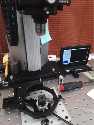
A Point Source Microscope (PSM) was mounted on a motorized vertical stage above a 25 mm diameter, 200 mm efl lens sitting above a plane mirror. A square black paper mask with an 8 mm diameter hole was placed over the lens as shown in the figure below to give an f/25 aperture.

BACKGROUND:

I was asked, “How well can the PSM find best focus of slow optical system?” In particular, could best focus be determined to ± 10 μm on an f/25 system? Conventional wisdom would say this is not possible as the depth of focus is on the order of λ(f/#)^2, something like 400 μm in this case. On the other hand, conventional theory claimed sub-micron microscopy in the visible was not possible until the invention of confocal microscopy. The answer for me was to try an experiment.

(The black ring mirror mount surrounding the lens and mask where used in another experiment.) The PSM had a 4x microscope objective attached.

After centering the lens to view the back focus in the center of the PSM video monitor, the PSM was scanned vertically over a range of about 1 mm while collecting and storing data about the reflected image every 4 μm for a total of about 264 points per scan.

The centroiding algorithm in the PSM looks at pixels more intense than a user set threshold. The threshold was set to about 125 out of an 8 bit range of 256. When the PSM is used for alignment, the centroiding algorithm calculates the center of gravity of those pixels above the threshold. The software also records the number of pixels above the threshold at each point in the scan. The shutter speed or exposure was user set so there were about 35 pixels above the threshold near best focus.

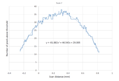
The limits of the 1 mm scan were then set to give a roughly symmetrical distribution of pixels around best focus so that a typical scan gave a curve in Excel like that below.

Using the curve fitting options in Excel, a quadratic curve fits well as expected. If the criterion for best focus is taken as the distance where there are the greatest number of pixels above the threshold, then taking the derivative of the equation and setting it to zero gives x = 0.2842 mm. The data are a bit noisy but the results look promising.

Much to my pleasant surprise, the other 9 repeated scans looked very much the same. The results are summarized in Table 1.

Table 1 The scan number, equation of fit to the number of pixels above threshold vs focus position and the position of best focus in mm

Ten scans through focus were taken under identical conditions, that is, over the same distance with the same threshold and exposure. The data from the scans were fit to second order polynomials as in the Scan 7 picture, and the coefficients of the fit are displayed in Table 1. Solving for the best focus position, defined as the position where there are the most pixels above the threshold gave an average best focus position of 0.2840 ±0.0020 mm.

These encouraging results must be viewed with two caveats; the test for finding best focus was a double pass test off a plane return mirror so single pass results will be less precise by a factor of two. The other caveat is the definition of what constitutes best focus, this may not be best focus in terms of best resolution for a particular spatial wavelength. However, it is a useful definition if it is desired to see if multiple examples of the same optical system behave similarly to a measurement of best focus.

The conclusion of this simple experiment is that the PSM can find best focus for an f/25 lens in double pass transmission with a standard deviation of 2.0 μm when axially stepped multiple times through the region of focus. Each scan took about 5 seconds, and the fitting and analysis of the data from multiple scans are easily automated

Customers purchasing a PSM often ask me if we offer mounting hardware for the PSM like x-y-z stages.

MY ANSWER HAS BEEN “NO”, BECAUSE THERE ARE SO MANY WAYS OF USING THE PSM THAT IT WOULD BE IMPOSSIBLE TO MEET EVERYONE’S DIFFERENT NEEDS.

IN FACT, THE ANSWER IS “YES!”

The centering station is a tall, motorized and encoded z stage with x-y lateral adjustments more than adequate to keep an image within the PSM field of view.

I use the centering station daily because it is so convenient.

Rather than attaching the PSM to an x-y-z mount as a first step, I simply move the lens or assembly to the centering station and I am ready for almost any type of lens measurement.

For any sort of measurement you might do on a classical optical bench, the centering station is a convenient and cost effective solution.

And being vertical, gravity is your friend.

Can the PSM find best focus of an f/25 optical system to less than ± 10 μm?

SOMEWHAT SURPRISINGLY, YES, TO ABOUT ± 2 ΜM.

You scan axially through best focus several times and plot the number of pixels above threshold versus scan distance.

The curve is quadratic and the derivative of the curve fit to the data gives the best focus position to even very slow systems.

The Axicon centering station and the associated LCS-PSM software make this an easy task.

The MicroFinish Topographer helped bring you this spectacular image of the sun.

The smoothness criterion on the Daniel K. Inouye Solar Telescope primary mirror was a scatter specification. This was a problem in two respects, the mirror substrate was Zerodur and the scatter angle was too close to specular to measure with a scatterometer. The near zero expansion Zerodur is a microcrystalline glass ceramic that scatters light when illuminated so a scatter test could not be used during polishing. Also, the scatter angle in the specification was so close to specular that the detector in a scatterometer partially obscured the scattered light path and could not be used even if the substrate did not scatter.

Kashmira Tayabala, et. al., “Use of the PSD and incident angle adjustments to investigate near specular scatter from smooth surfaces”, Proc. SPIE, 8838 (2013) showed that the MicroFinish Topographer (MFT) could measure surface roughness over sufficiently long distances to infer the magnitude of the near specular angle scatter. Given this insight, the MFT was used to show the Inouye Solar Telescope primary met the near specular angle scatter specification, Chang Jin Oh, et. al., “Fabrication and Testing of 4.2m Off-Axis Aspheric Primary Mirror of Daniel K. Inouye Solar Telescope”, Proc. SPIE, 9912 (2016).

A combination of the Auto Gain function of the Point Source Microscope (PSM) and the use of an Axicon grating make centering of severely misaligned lenses easy.

The lenses in the cell are misaligned far enough that light in the center of the aperture barely makes it through the lens.

The PSM video screen displays a partial set of rings produced by a combination of the PSM and Axicon grating. The orientation and curvature of the rings indicates how the lens cell must move to center it with respect to the Axicon grating axis. Note that the PSM objective focus is at an arbitrary height about the lenses, not at a back focus, or center of curvature of one of the lens elements

The first video picture (left) shows the partial ring pattern with the lens misaligned as in the picture above. As the lens is moved by the screws it is clear the centering gets better (middle). The next picture (right) shows the center of the Axicon grating pattern now in the field of view of the video screen. The magenta crosshair is barely visible in the center of all three pictures and is the reference for centering.

The bright spot in the center of the Axicon grating pattern is much more intense than any of the rings. This intensity forces the Auto Gain function to reduce the gain and shutter exposure time so there are no saturated pixels in the display so the final centered pattern looks like the picture on the left side above where only the center spot and first few rings are visible centered on the crosshair. The picture on the right is a blow up of the one on the left to make the crosshair and scale bar easier to see.

The full screen shot shows that the central spot is centered to less than 1 μm. Also, the Auto Gain was turned off so that more detail in the rings is visible.

The centering was accomplished as fast as the adjustment screws could be turned. This contrasts with the conventional situation where the centering objective must first adjusted to focus at a back focus or center of curvature so there is sufficient focused intensity to view on the video screen. Then the lens cell is moved around to find the focused spot that is lying outside the field of view of the microscope. This is often the most difficult part of the alignment, finding the focused spot when there is no signal on the detector until you are within the field of view of the objective, typically within 0.5 mm when using a 10x objective.

With the Axicon grating the alignment is much faster than conventional methods and less tedious because there is a useful centering indicator even though the lens system is vastly decentered. The lack of tedium makes the work of centering pleasurable rather than a chore.

Recently a customer was using the Point Source Microscope (PSM) to align a slow, singlet objective lens and find its focus. 

The customer had a plane retro mirror behind the objective and should have seen a nice round spot at best focus. Instead, he saw a vertical line image as in the following screen shot of the PSM computer display.

The customer knew the PSM was working correctly because he did get a small, round image when he focused at the center of a good grade steel ball. He also knew the lens was correctly aligned to the PSM because he had used the PSM in the autocollimator mode and had reflections from both sides of the lens centered on the PSM electronic crosshairs.

When he did decenter the PSM and looked at the reflected image on a white card he saw a line image. In addition, when he tried to refocus over a 25 mm range he could not find a circle of least confusion. All this pointed to a severely astigmatic return wavefront since the lens was from a trusted vendor. The test set up is shown in the picture below. The rear of the PSM is in the foreground and the objective is at the far end of the optical table with an undersized plane mirror behind it.

I suggested that it might be the small, plane retro return mirror was not flat because the mount was squeezing it. He assumed this was not the case but said he would check.

Not long after I got an email with this picture showing the great improvement in the image after remounting the return mirror.

Clearly, the problem is not completely solved, but the image is many times better than before and the source of the problem isolated. The PSM laser diode source is in the maximum intensity mode that makes the image larger than it should be due to saturated pixels in the camera, and there is still some astigmatism in the wavefront or the spot would be round. The red line just under the horizontal line image is 100 μm long for scale. The lens was about 2 m from the PSM so the roughly 250 μm long image has an angular width of about 5 seconds of arc. The height of the image is slightly more than one would expect due to diffraction.

This is just one example of how the PSM can spot a problem in a test set up before the problem becomes serious. The problem might be serious due to the time it takes to track down its source, or if the problem is not fixed, the issues it will create farther downstream if not corrected at the source.