We describe a method of calculating the vertex radius of an off-axis parabolic segment using a three ball spherometer to measure the sag. The vertex radius is found by solving a set of six simultaneous, non-linear equations for the three coordinates of one of the ball centers and the corresponding three coordinates of the point of tangency of the ball with the surface.
1. Introduction
Three ball spherometers are the 1” micrometers of an optical shop and have been used for over 100 years to measure the radii of spherical surfaces.1,2 The radius of curvature of a spherical surface can be calculated from a simple, three term formula that includes the measured sagitta, or sag, the distance from the central micrometer or indicator and the center of the balls and the radius of the balls.3,4 Until recently, in spite of the simplicity of the formula that includes a square in one term, spherometers were sold with tables that converted sag readings into radii because optical shop personnel often did not have the skills or time to solve the formula. With the advent of pocket calculators it is now easy to solve the sag equation.
The sag equation is rather simple because the spherometer balls touch the surface at normals to the surface, and for a sphere these go through the center of curvature of the sphere and through the centers of the balls on the spherometer. In the case of an aspheric surface this is not so; the ball centers still lie on the normals to the aspheric surface but the normals do not go through the center of curvature of the asphere. The solution to this problem requires the solution of six non-linear, simultaneous equations, again something not easily undertaken even by rather mathematically adept optical engineers. However, with the advent of equation solvers such as the “Solver” function in Microsoft Excel, solution of these simultaneous equations is straight forward and fast. This is the problem we will illustrate.
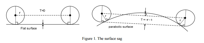
2. Measured surface sag (T)
The measured sag, T, is the difference between the spherometer indicator reading when the spherometer is sitting on a plane surface, Fig. 1 (left), and when the spherometer is resting on the aspheric surface to be measured (right). We have shown the case for a convex surface but identical conditions hold for a concave surface with the exception that the sign of the indicator movement is opposite.
3. Geometry of the three ball spherometer
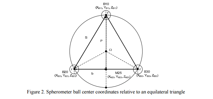
Referring to Figure 2, the spherometer has three balls on the points of an equilateral triangle. D is the diameter of the circle through the centers of the balls, S is the length of the side of the triangle and the distance between ball centers, P is the height of equilateral triangle, Ω the distance from the center of the triangle to the balls and r is the radius of the balls. B10 is the center of the ball located on the meridional plane of the parabolic segment and the vertex of the parabola lies above this ball. B20 and B30 are ball centers located symmetrically with respect to the meridional plane. Relationships of the sides of the spherometer are given below.
4. Geometry of the spherometer resting on the parabolic surface
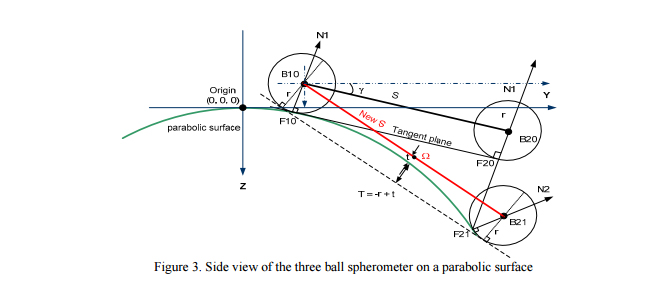
We use a Cartesian coordinate system where z is the axis of symmetry of the paraboloid and y lies in the meridian plane. The origin is coincident with the vertex of the parent parabolic surface. When the spherometer is first set on the parabolic segment we place ball B10 on the meridional plane with the tip of the indicator approximately centered on the segment. At first we know only that XB10 = 0, YB10 is approximately P less than the center of the segment and ZB10 is r higher along the normal to the surface than where the ball touches the surface, ZF10 = YB10^2/(2Rv) where Rv is the vertex radius of the parabola.
Referring to Fig. 3 we see the spherometer in two states, the final one (subscript 1) sitting on the surface and an initial one (subscript 0) where the calculation is begun. We start by assuming the plane of the three spherometer balls is perpendicular to the normal to the surface at F10. This allows us to calculate a starting position for B20, and by shifting the plane of the ball centers downward by r, the starting position for F20.
Then we assume the spherometer is iteratively rotated down to the surface about the center of B10. The point of contact, F10, will not change nor will the dimensions of the spherometer. However, as the spherometer is rotated so the other two balls rest on the surface the calculated dimensions of the spherometer will change. Since the spherometer dimensions cannot change we have a method of solution by simultaneously solving the six equations below for the centers and points of tangency of the floating balls.
5. Calculation of points of tangency to the parabolic surface of the equilateral triangle base
The six unknown variables are
and they are found by solving six equations simultaneously. The six equations are
The relationship of the ball center to the point of tangency along the normal to the surface
where α, β and γ are the angles of the normals to the surface at F21. Finally the distances between the balls
Once the six unknowns are found it is straight forward to find the coordinates of the center of the spherometer and project the indicator down to the surface of the parabolic segment normal to the plane of the ball centers. In general, the tip of the indicator will not hit the center of the segment exactly and a new value will have to be used for YB10 and the calculation repeated until the tip is close enough to the desired location. Notice too that we have calculated the sag assuming the vertex radius is correct. If the measured sag is different from the desired, the Rv in eq. 5 must be changed until the results match the measured sag.
6. Summary
We have shown how the sag of an off-axis parabolic segment as measured with a three ball spherometer may be used to determine the vertex radius of the segment. While this is not as easy as for a spherical surface, the calculation is well within the capabilities of an optical engineer with access to iterative equation solving software.
7. References
1. Grubb, H., Nature, 34, 85 (1886)
2. Ritchey, G. W., Smithsonian Contributions to Knowledge, 34 (1904)
3. Horne, D. F., “Optical Production Technology”, p. 324, Crane, Russak & Co., Inc., New York 1972
4. Malacala, D. “Optical Shop Testing”, p. 818, 3rd ed., Wiley-Interscience, 2007.
Auto-stigmatic microscopes (ASM) are useful for bringing centers of curvatures of lenses and mirrors to the centers of balls used as part of an alignment fixture. However, setting up the fixture to get the balls used for alignment in a straight line to represent the optical axis generally requires another piece of equipment. We show that within a practical range, the autocollimation mode of a modern ASM can be used to align balls to an axis with about the same precision as they could be aligned with an alignment telescope, or laser tracker. As a lead in to this topic, we discuss our meaning of alignment, the means of positioning optically important features such as centers of curvature and foci to the coordinates specified on assembly drawings. Finally, we show a method of using an ASM along with other tooling to align a toroidal mirror using its foci.
1. INTRODUCTION
1.1 Definition of alignment
In a paper on alignment we should start by defining alignment. Every optical system is built to a design. First, there is the optical design, and it is used by a mechanical engineer to design a barrel or optical bench into which the lenses and mirrors are held. Throughout this design effort, the optical elements are assumed precisely located where the design specifies. It isn’t until the optical bench and elements come together that the issue of alignment comes up. It is at the assembly stage where the elements must be located precisely where the design or drawing specifies. This is alignment, getting optical features such as centers of curvature, axes, and foci positioned precisely as the design or drawing indicates.
In order to get the optical features located precisely, an instrument is needed that can sense the optical feature in question precisely. The same instrument, in conjunction with mechanical tooling, must also sense mechanical datums in the lens barrel or optical bench since the axes and foci of the optical system must be positioned precisely relative to specific mechanical features called out in the design. For example, the design may call for the optical axis of a system to be concentric with the outside of the cylindrical barrel of the assembly. Thus there must be a way of locating both the optical axis of the optical elements and the mechanical axis of the cylindrical barrel to assure coincidence of the axes.
1.2 Autostigmatic microscope
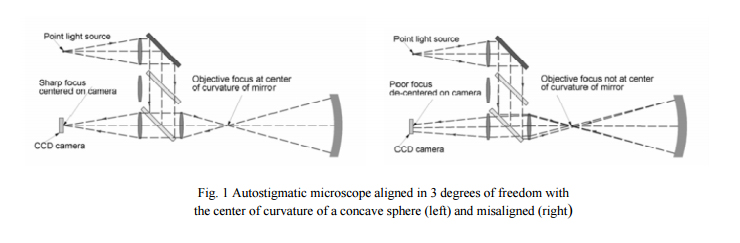
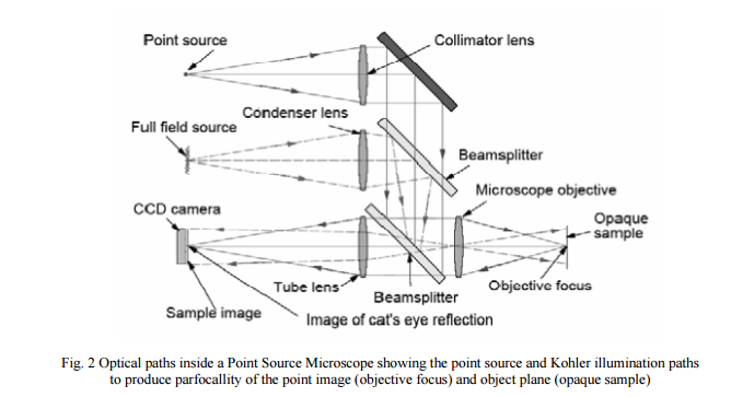
An instrument that can define both optical and mechanical datums in conjunction with some simple mechanical tooling is an autostigmatic microscope1 . In simplest terms, an autostigmatic microscope is a microscope that has a point source of illumination that is conjugate with a set of crosshairs in the image plane, either real physical crosshairs in an eyepiece or electronic crosshairs on a video display. If the autostigmatic microscope is perfectly aligned to the center of curvature of a sphere, the reflection from the sphere will form a well focused point image centered on the crosshair, that is, it defines 3 degrees of freedom (DOF). If the microscope is not well aligned the spot will be out of focus and shifted laterally from the crosshairs. Fig. 1 shows the typical optics of an autostigmatic microscope both aligned and misaligned with a concave sphere.
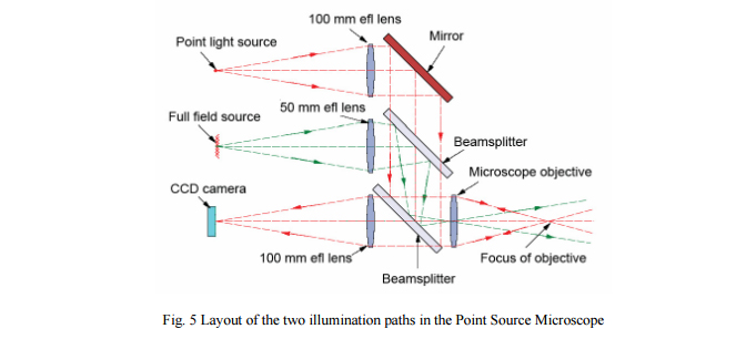
In order to make the autostigmatic microscope more useful, the addition of full field, or Kohler, illumination is helpful so the microscope can image as an ordinary microscope does. If the focal plane of the imaging arm and the autostigmatic focus are the same, the instrument is even more useful in that both types of illumination can be used simultaneously as will be illustrated in the first example of its use in section 2. A microscope with these features that is commercially available is called a Point Source Microscope2 and the optical paths in the microscope are shown in Fig. 2.
2. ALIGNMENT OF A STAGE COINCIDENT WITH AN AXIS OF ROTATION
2.1 Some definitions
As a first example of alignment with an autostigmatic microscope, we will consider the alignment of a single axis linear stage with the axis of a rotary bearing. The specific example will be a vertical stage over a rotary table used for centering lenses, but the example is just as applicable to the alignment of a lathe headstock with the lathe bed and tailstock center.
As with the term alignment, it is best to start with a definition or two. Since we are aligning an axis we should note that an axis is a line and a line is defined by two points, or a point and an angle in two planes, in other words by four DOF. Rotation about the axis and distance along the axis are not defined.
Another term used in conjunction with axes of rotation is centering and this can be confusing since there can be two meanings to centered. For a point, or spot, to be centered on an axis of rotation it is stationary when the axis is rotated. For the axis to be centered on the microscope, the axis must lie on the microscope axis, or crosshairs. The illustration in Fig. 3 helps explain the difference in the two concepts assuming a rotating table.
In the upper left of Fig. 3 the spots of light produced by the autostigmatic microscope move in a circle as the rotary table revolves about its axis. This means the light spot does not lie on the axis of rotation. In the lower left, the light spot is centered on the axis of rotation, but the axis of rotation is not centered on the microscope axis, or crosshairs. In contrast on the upper right, the spots are rotating about the microscope axis but are not centered on the axis of rotation, while in the lower right, the spots are both centered on the axis of rotation and that axis is centered on the microscope axis or crosshairs. In short, if the spots are moving in a circle, the spots are not centered on the axis of rotation meaning the center of curvature from which the spots are reflecting does not lie on the axis of rotation of the rotary table.
The same concept applies to centering an object in the microscope field of view. Consider the crosshair target in Fig. 4 that is imaged by the microscope. One end of the crosshair is indicated by a circle to show that the crosshair rotates as its center traces out a circle about the axis of rotation of the rotary table.
As seen in the lower left view of Fig. 4, the crosshair will rotate as the axis is rotated but the center of the crosshair remains stationary in the field of the microscope indicating that the crosshair lies on the axis of rotation but is not centered on the axis of the microscope while it is in the lower right view. The two types of centering require two physically different operations; to center the spots or crosshair on the axis of rotation, the optical surface must be translated or tilted relative to the axis of rotation. To get the axis of rotation to lie on the microscope axis either the microscope must be moved to the axis, or the axis of rotation translated or tilted to make it coincident with the microscope axis or crosshair.
2.2 Alignment of an axis
Now to the alignment of the vertical stage to the axis of the rotary table. Fig. 5 illustrates the situation. There is a rotary table in the lower part of the Figure and a vertical stage to the right. The Point Source Microscope (PSM) is shown in two positions on the stage, one focused on a target on the table using the imaging light source and one at the center of curvature of the plano concave lens lying on the table. These two foci of the PSM are the two points on the line defining the axis of the stage since the PSM is physically tied to the stage. The axis of the table is virtual because it cannot been seen, but it is made real by use of two simple fixtures, a crosshair target on the rotating table defining one point on the axis and the plano convex lens defining the other.
To align the axis of the rotary table to the axis of the stage as defined by the PSM focus, we must both make the target crosshair and the reflection from the concave surface stand still in space. This is accomplished by translating the target and lens, separately, relative to the table top. The target can be a piece of paper with the lens sitting on top. When the PSM in the imaging mode is focused on the paper the situation will typically look like the case in the upper left of Fig. 4. The target must be decentered relative to the rotary table top until it looks like the case in the lower left of Fig. 4. Then the target crosshair lies on the axis on the rotary table.
Similarly, at the center of curvature of the lens, the situation will look like the case in the upper left of Fig. 3 when the PSM is focused at the center of curvature using the autostigmatic mode. If the vertical stage is very decentered, the stage may have to be translated to get the return image in the field of view of the microscope, but the real task is to make the reflected spot cease to move as the table is rotated, that is, to achieve the case shown in the lower left of Fig. 3.
Once the crosshair and spot are centered, that is, not moving except in the case of the cross, rotating about the center of the cross, it is then necessary to translate and tilt the stage until the cross and spot both lie on the crosshairs in the microscope. When the alignment is finished the crosshair target will look like the case in the lower right of Fig. 4 and the spot will look like the lower right of Fig. 3. It is important to make these adjustments in the correct order, center the targets on the rotary axis first and then adjust the column. Further, remember that the target errors are seen doubled due to the rotation, and in the case of the spot, reflection. Do not try to make the full correction all at once. You will overshoot every time and the alignment will take at least twice the time it should. Make the adjustments in fractions of what it looks like the translation needs to be.
Notice, too, this alignment could not be done without some simple fixturing to “realize” datums that are virtual without the fixturing. In general, the most useful fixtures are spherical surfaces, physical realizations of points, and next most cylinders, realizations of lines. These make the most precise realizations because if lens surfaces or high grade spherical balls are used, their centers can be located to <1 μm. With images of crosshairs, it is difficult to use centroiding algorithms to achieve micron centering, but 10 μm centering is easy with images.
3. ESTABLISHING AN AXIS
In this example, we will describe how to use an infinity conjugate autostigmatic microscope to establish an axis. This is important because the majority of optical systems have a single axis of symmetry and alignment for these systems means having the centers of curvatures all lying on a common axis. In passing, the easiest way of establishing an axis is to use a good rotary bearing like in the previous example. However, there are many times when such a table is not available or the optics are too large to put on a rotary table.
For the alignment of a system with a single axis, fixtures or datums have to be positioned at precise locations along the axis. The lateral positions are tighter than the axial locations, but the axial locations still need to be carefully controlled. The most common way to do this alignment is with an alignment telescope3 , but it is a tedious proposition and almost always requires two people, one looking in the eyepiece and one making the adjustments to the fixtures.
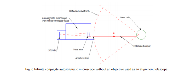
There is an alternative that works well over distances from about 0.5 m to 3 m. That is, remove the objective from the autostigmatic microscope and use the collimated beam projected by the 6 mm aperture. When the collimated beam reflects off a spherical surface, the return wavefront is nearly spherical, and for that part of the wavefront returning through the aperture on the microscope it is perfectly spherical assuming a good grade spherical ball. This situation is like that shown in Fig. 6 where a steel ball is used to maximize the reflected light.
The spherical wavefront reflected off the ball will have a radius of curvature of approximately the distance from the microscope to the ball. Assume for this example the distance is 1 m and the ball is 25 mm in diameter. The PSM has a 6 mm aperture and a 100 mm tube lens. This means the return wavefront will produce a spot about 0.6 mm on the 1/3” CCD detector that is 3.6 mm in the short direction. While this is not a perfectly focused spot, the centroiding algorithm in the PSM software works just as well on out of focus images as well focused ones. The limit here is that the entire spot lie on the CCD. In this example, the shortest distance from ball to PSM would be 250 mm to keep the image from being bigger than the detector. If a shorter distance were needed, the 6 mm aperture could be stopped down. Also, short distances mean plenty of light gets back through the aperture stop.
The far distance is limited by the light available but has the advantage that the spot on the CCD is smaller. For the example, the 6 mm collimated beam is spread into a cone of 0.235 steradians. At a 1 m distance, the 6 mm aperture subtends just 36 μsteradians, or collects just 1.5×10⁻⁴ of the reflected light assuming a top hat intensity distribution. On the other hand, the PSM has an intensity dynamic range of about 1×10⁵ . Thus a dynamic range at a distance of 3 m or more is perfectly reasonable.
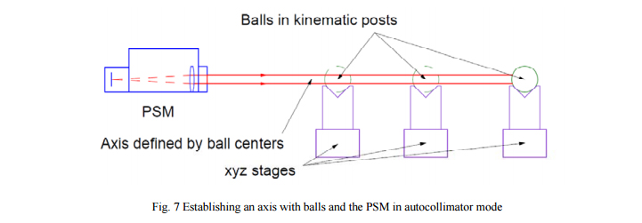
Figure 7 shows the PSM used in the autocollimator mode to align a set of balls on a common axis. Here the farthest ball is aligned first. A post such as used to position lens mounts can be used as a kinematic locator for the ball. The post is on an xyz stage and the stage is adjusted until the reflection from the ball is centered on the PSM display. Subsequent balls are similarly adjusted. The axial spacing is set using an inside micrometer.
There are several advantages over using an alignment telescope in addition to those already mentioned. The collimated beam is bright enough to see under ambient lighting so it is easy to set up the initial alignment, the balls are easier to use than crosshair targets needed with an alignment telescope, the set up has no moving parts in the alignment instrument and there is nothing to focus. Finally, the centroiding is completely objective.
In terms of precision, the centroiding algorithm has a sensitivity of just under 1 arc second, or ~5 μradians. Even with out of focus images on the detector experience has shown this to be the case. The means that balls aligned using this method can be positioned to about ±5 microns at the distance of 1 m. Over the range where sufficient light reaches the detector this sort of precise is on the order of that achievable with a laser tracker.
4. ALIGNMENT OF SYNCHROTRON MIRRORS
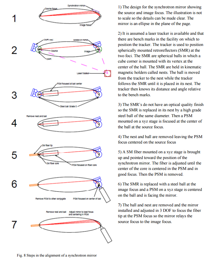
The final example is one that I have not had the opportunity to try out but is illustrative of a technique that could be applied to many situations where high precision alignment is required in a multi-dimensional space. Further, it shows how the autostigmatic microscope can be used along with other sophisticated optical tooling such as a laser tracker4 to increase the value of both the tracker and the microscope. The whole example is laid out in Fig. 8 and the various steps will be described in the text, one after the other. This is again an example of how there is a particular sequence of steps that must be gone through to achieve the final alignment.
The synchrotron mirror is5 almost plane and thus has the same DOF as a plane mirror, rotation about the axes parallel to its face and translation perpendicular to its face. Using these 3 DOF the mirror is adjusted so the light from the fiber tip is focused at the PSM focus. The focus will be a line normal to the page and have a width limited by diffraction set by the apparent width of the mirror looking into it at grazing incidence in the plane of the page. The other 3 DOF are set using mechanical datums on the mirror and the structure holding the mirror.
In this example we have tried to demonstrate the use of the autostigmatic microscope with other optical tooling used in large optical projects. The SMR’s used by the laser tracker are completely compatible with the use of steel balls used in other autostigmatic microscope applications. The imaging aspect of the PSM permits its use in the location and centering of an optical fiber tip that will then be used as a point light source at one conjugate of the system. Finally, the PSM can be used to detect the focused image coming single pass through the optical system to align the synchrotron mirror.
5. CONCLUSIONS
We have first set out a working definition of optical alignment as determining the location of an optical, as opposed to a mechanical, feature, and then moving that feature to the location specified in the design of the optical system. Then we have given a simple example of the alignment of a center of curvature to an axis of rotation to show the difference between alignment of the feature to the axis of rotation, and the alignment of the axis to the instrument making the measurement. This is followed by an example of using an infinite conjugate autostigmatic microscope to align a series of spherical ball targets in a straight line. Finally, we show how to use an autostigmatic microscope in conjunction with a laser tracker to systematically align a synchrotron mirror using the mirror’s two foci.
Precision lens centering is necessary to obtain the maximum performance from a centered lens system. A technique to achieve precision centering is presented that incorporates the simultaneous viewing through the upper lens surface of the centers of curvature of each element as it is assembled in a lens barrel. This permits the alignment of the optical axis of each element on the axis of a precision rotary table which is taken as the axis of the assembly.
1. INTRODUCTION
Lens centering is a crucial step in the manufacture of rotationally symmetric optical systems. For optical systems to deliver maximum performance the optical design must be superior, the lens elements accurately manufactured and the elements well centered in a barrel. With experienced designers, sophisticated software and vast computing power, superior designs are easier to produce than in the not too distant past. With phase shifting interferometers and mature computer controlled polishing it is possible to produce optical surfaces accurate to a few nm rms or better.
In order to take full advantage of an excellent optical design and well manufactured optical surfaces the lens elements must be well centered in the assembly. Without a careful and accurate job of centering the money put into design and polishing will be lost. This paper discusses how to do a superior job of lens centering by simultaneously sensing both centers of curvature of each element from above as the element is placed in the lens barrel and the barrel is rotated about its axis. Each element is adjusted in tilt and decenter until there is no motion in either center of curvature.
To demonstrate this procedure we will first discuss the definition of centering and give a specific lens design as an example. Then we will show how to locate the centers of curvature of the lens surfaces looking from one side of the lens only. The instrument used to optically locate the centers of curvature, an autostigmatic microscope that we have called the Point Source Microscope (PSM), will be described and an example of how it would be used to find the center of curvature for each lens surface will be given.
Finally we discuss how the tilt and decenter of the surfaces affect performance of the lens system and how sensitive the PSM is to these centering errors to give a feel of the performance improvement using this superior centering technique. This leads directly into the conclusions.
2. DEFINITION OF CENTERING
2.1 Optical axis of a lens element
The optical axis of a lens is the line between the centers of curvature of the two surfaces. It is a paraxial property that is seldom given any thought but is the basis for this discussion. Aspheric surfaces do not change the definition. If the whole aspheric surface produces too much spherical aberration to center on the reflected return image the surface may be stopped down to effectively make the surface paraxial.
There are several things to note about this definition; it is completely independent of the mechanical features of the lens such as the periphery or seat, and the definition is incomplete without considering both lens surfaces because a single sphere has no intrinsic axis. If a lens is poorly centered its periphery is not concentric with the optical axis nor is its seat perpendicular to the axis, but it still has a well defined optical axis.
In terms of the larger aspects of a lens system, if both object and image lie on the optical axis of the lens system it is being used on-axis. If one or more elements within the lens system are decentered it becomes difficult to define the axis of the system. Probably the best definition then is the angle the lens must be tilted to produce the best image, that is, how must the lens be tilted about the line joining object and image to produce the best image.
2.2 An example lens system
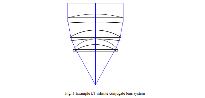
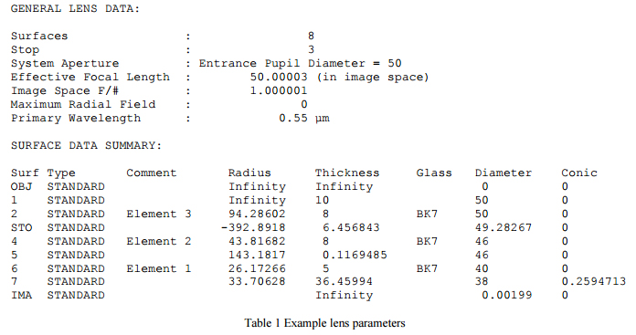
To demonstrate the ideas about centering we give the design of a three element, all BK7, f/1 infinite conjugate lens with one aspheric surface. The design is shown in Fig. 1 and the parameters given in Table 1. The design has about 0.035 waves P-V of spherical aberration and is 0.0075 waves rms at the design wavelength of 0.55 µm.
3. LOCATING THE CENTERS OF CURVATURE OF THE LENS SURFACES
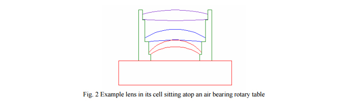
Before looking at the centers of curvature of the lenses we show the three lens elements in their cell (see Fig. 2) to give a feel for the physical constraints on centering. The cell is sitting on top of an air bearing rotary table and has been adjusted so there is zero runout or decenter and no tilt, that is, the axis of the cell is coincident with the axis of the rotary table. It is further assumed there is no error in the table bearing, an assumption good these days to 50 nm sorts of dimensions.
It is clear from Fig. 2 that all optical sensing of the centers of curvature of the elements must be done from above the lens system. While rotary tables are available with through holes1 and use of the underside of the lens may make some examples easier, particularly in volume production, we show there is no need to view the lens from the bottom.
It is clear how to locate the centers of curvature of the upper sides of the lenses, the centers of curvature lie a distance equal to the radius of the upper surface below the lens element in question. A positive lens with a long working distance, or back focal length, will have to be placed above the example lens system. As a reasonable choice a 100 mm efl lens could be used because the longest convex radius is 94.286 mm on the upper surface of Element 3.
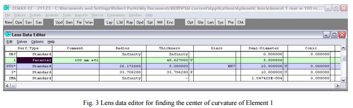
Now we will use this positive lens along with a lens design program such as Zemax2 to find the apparent location of the center of curvature of the rear surface of each lens element looking through the upper surface. For Element 1, the first one that will have to be inserted in the cell, the Lens Data Editor is set up as in Fig. 3.
The object is set at infinity feeding the paraxial (perfect) 100 mm efl lens that is surface 1. The distance (thickness) between the paraxial lens and the front surface (line 2) of Element 1 is the unknown (or variable) we must find. On that line (2, also the stop in the system) is the radius of the upper surface, 26.172 mm, the thickness of the lens, 5 mm, and the material, BK7. The next line (3) is the rear surface of Element 1 with a radius of 33.70628 mm. If the light is to strike that surface at normal incidence, the condition necessary when a point source is at the center of curvature, the light must come to focus a distance equal to the radius of the surface farther to the right. That is why the thickness for the rear surface is also 33.70628 mm as is assured by using a pickup (P) from the radius column.
The next, or image, line shows the light is focused at this distance because the diameter of the image is very small when the thickness from the paraxial lens to the front surface is 48.627 mm, a value found by using the design optimizer.
Notice the thicknesses do not add to 100 mm showing the effect of refraction at the front surface. Another way of finding the distance between the center of curvature and the front surface of the lens is to use paraxial ray tracing to find that
Notice this is just the paraxial lens focal length minus the paraxial lens to front surface thickness of 48.627, or 51.373. The 5 µm difference between the results can be accounted for by not using a small enough aperture size to make the lens design optimizer give a truly paraxial result.
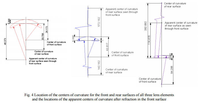
Fig. 4 shows the results of using this same technique on all three lens elements in the system. Notice for Element 1 that the distance from the rear surface to the focus, 46.373, plus the lens thickness, 5, and the distance from the lens front surface to the paraxial lens, 48.627, add to 100 mm, the efl of the paraxial lens. Also shown are the physical centers of curvature of the two surfaces. The same logic holds for the other two elements but in these cases the center of curvatures of the rear surfaces after refraction are above the front surface by 556.182 and 106.416 mm for Elements 2 and 3, respectively.
Although the example lens system does not have a concave front surface it is obvious that the center of curvature of this surface would be above the surface by the radius of the front surface. The method for finding the location of the center of curvature of the rear surface after refraction in the front is the same as for this example. Now that we have shown how to locate the centers of curvature of both lens surfaces from above the lenses we show how to use the Point Source Microscope (PSM) to view these locations.
4. POINT SOURCE MICROSCOPE (PSM)
The PSM is a video metallographic, or reflected light, microscope using Köhler illumination to provide uniform intensity over the field of view. In addition, the PSM has a point source of illumination produced by the end of a single mode fiber pigtailed to a laser diode that is conjugate to the microscope object plane as shown in Fig. 5 below. This point source of light makes the PSM into an autostigmatic microscope, and it is this feature that is used to view the centers of curvature of lens elements during centering.
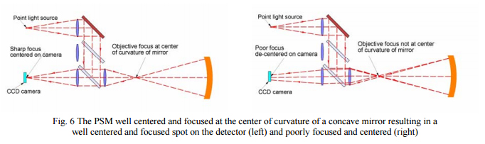
When the point light source is used and the focus of the microscope objective is conjugate with the center of curvature of a lens element or mirror surface the light will strike the surface at normal incidence and be reflected back to the microscope objective focus and on to the CCD detector where it can be viewed on a monitor. When the alignment with the center of curvature is precise in lateral position and focus the return spot will be a well focused and centered on the detector. If the alignment and focus are less than ideal the spot will be defocused and decentered as shown in Fig. 6.
It remains to show how two PSMs can be set up to view both sides of a lens element simultaneously so the optical axis can be established and aligned. It is also obvious that there are limits as to how well lenses need to be centered and the PSM can be used to tell if the centering is good enough by measuring the excursion of the return spot of light as the rotary table is turned.
5. VIEWING BOTH CENTERS OF CURVATURE SIMULTANEOUSLY
5.1 Scheme for simultaneous viewing
Because the optical axis of a lens element is the line joining the centers of curvature and it is that axis that must be aligned to both the cell axis and the other elements within the lens system it is most expedient to view both centers of curvature simultaneously during centering. Although the centering operation can be done be viewing just one center at a time it is very tedious to do it this way because the alignment of one center may, and usually does, disturb the centering of the other.
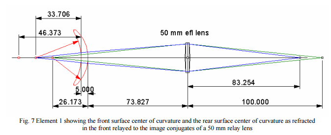
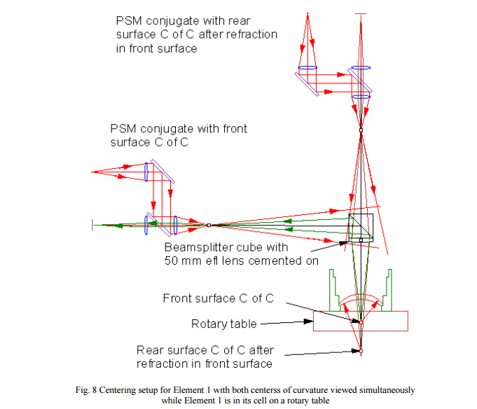
Going back to our example lens we look at Element 1 first. In Fig. 7 we show just the location of the upper or front surface center of curvature and the rear surface center after refraction in the front surface because these are the two centers we see with an autostigmatic microscope
Now instead of using a 100 mm efl lens at infinite conjugates we use a 50 mm efl lens at 1:1 finite conjugates to relay the front surface center of curvature to the right side of the 50 mm lens. However, this same lens can be used to relay the rear surface apparent center of curvature with an object conjugate of 125.20 mm to the right side with an image conjugate of 83.254 mm accomplishing just what we wanted to do, image both centers of curvature simultaneously. It now remains to separate the centers so they can each be viewed without having to move a PSM.
This is most easily accomplished with a minor modification to the layout in Fig. 7, the introduction of a beamsplitter with a 50 mm efl lens cemented to it so there is only one optical component above the lens element being centered. The setup will then look like that in Fig. 8 where the optical paths of both PSM’s are shown. We have neglected the slight axial shift in the conjugates due to the optical thickness of the beamsplitter as well as the small introduction of spherical aberration it will produce. In practice the f/number of the cone of light used for centering is so narrow that the exact axial position and small amount of aberration is not critical. Further, all the conjugate calculations have been first order, or paraxial, so they are not exact but close and quite good enough for real implementation because what we are ultimately interested in is whether the relayed return spots from the centers of curvature move or not as the rotary table is turned.
5.2 Modification for viewing with two autostigmatic microscopes
Fig. 8 is rather busy but it shows the entire setup for centering Element 1. The two PSM’s send out cones of light that somewhat over fill the beamsplitter/relay lens combination and the relay lens serves as the stop as it sends converging beams of light to both the center of curvature of the front surface and to the center of curvature of the rear surface after the light has been refracted in the front surface. The light reflects off the front and rear surfaces of the lens and retraces itself back into the two microscope objectives. Both reflected light beams enter both objectives but the beams from the incorrect conjugates are so far out of focus that very little light reaches the detector and is inconsequential. Only light from the correct conjugate is well focused and bright on the detector of that PSM.
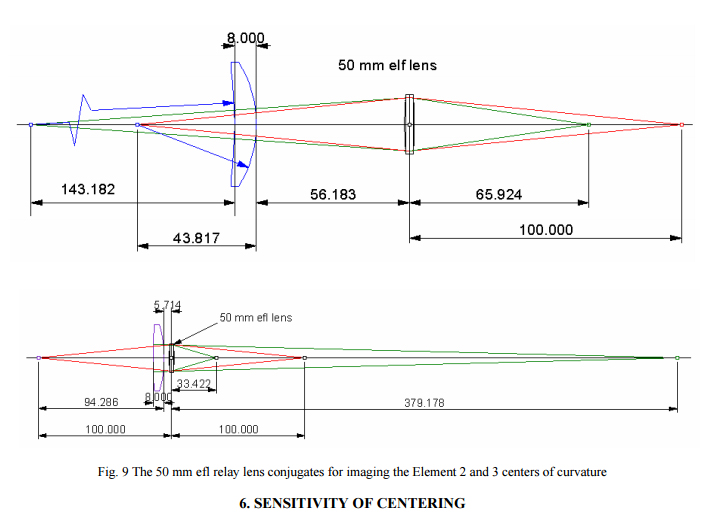
Similar setups work for the other two lens elements even though the rear surface centers of curvature appear above the front surface. Fig. 9 shows the conjugates for these two elements using the same 50 mm efl finite conjugate lens. In this example it just turned out that the same focal length lens could be used for all three elements. In general this will not be the case but a relatively few beamsplitter/relay lens combinations can be used for practically any lens element that needs centering. In fact, the relay lens is only 5.714 mm in from of Element 3 in Fig. 9, a distance that may be too close for comfort. A 60 or 75 mm efl relay lens could have been used just as well without much increase in the total dimensions of the measurement setup. Obviously all the relay lens conjugates would differ from the example.
It is further clear that the relay does not have to be used at 1:1 conjugates in one of the cases. The options for finding suitable conjugates is almost limitless, something that is a possible drawback in finding good conjugate solutions. However, it does show the flexibility in this system of simultaneous conjugate viewing. Along the same line the PSM does not have to be used with expensive microscope objectives since this application does not call for full field imaging. Inexpensive, longer focal length doublets can be mounted in lens tubes and mounted to the PSM using objective adapters. The beamsplitter would still have to be used but all the optical power would be in the PSM itself.
6. SENSITIVITY OF CENTERING
6.1 Theoretical considerations
Now that we have seen how to view both centers of curvature simultaneously we need to ask how sensitive are the PSM’s to tilts and decenters of the three lens elements in this example. For the front surfaces this is easy; if the surface is decentered 1 µm, the return spot will move by twice that because of the doubling on reflection. When the lens is rotated 180º with the rotary table the lens is decentered in the opposite direction so the total spot motion is 4 µm for a 1 µm decenter from the rotary table axis of rotation. Depending on the objective used, and the 5x would be typical for centering operations, there is another factor of 2.5 so the image motion at the detector is 10 µm. The detector has 4.65 µm pixels and can centroid to 0.1 pixels. Working backwards gives us a theoretical sensitivity to front surface decenter of about 47 nm.
Regarding rear surface decenters, clearly a front surface decenter will affect the apparent decenter of the rear surface. Rather than do a lot of calculations the pragmatic approach is to center the front surface first and then the rear surface decentered will not be affected except by a scale factor.
For tilts the sensitivity is linearly proportional the radius of curvature (or apparent radius) of the surface in question. Working backwards from the above example we find the sensitivity to tilt about 10 seconds of arc per mm of radius. Thus if a concave surface had a radius of 10 mm the PSM would be sensitive to a 1 second tilt of the surface and to a 0.1 second tilt if the radius of the surface were 100 mm.
It may be asked what is the effect of a tilt or decenter on the lens performance. A tilt displaces the chief ray so the lenses following the tilted element are in effect decentered. A decentered lens deviates the chief ray from the optical axis making the lenses following appear to be tilted. This is nicely shown in a recent paper by Burge3.
6.1 Practical considerations
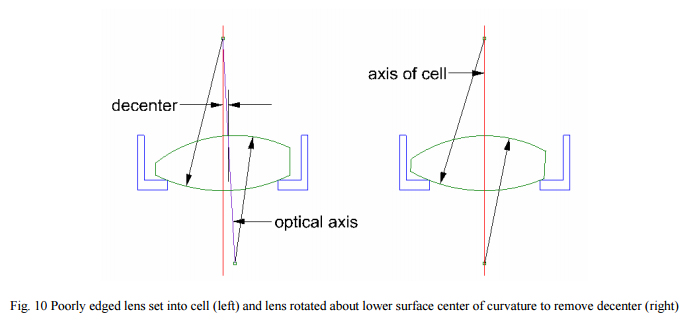
Now it is time to look at the real situation in most instances in terms of lens edging and assembly in a cell. We will first look at assembly to gain an insight as to what we need to look at in terms of edging tolerances. When a lens is set in a cell the lower spherical surface seats on a step shaped land that was machined into the cell that is concentric with the axis of the cell in the radial direction and perpendicular to the axis in the axial direction as shown in Fig. 10. In a perfect world where there are no burrs or contamination on the seat this arrangement assures that the center of curvature of the lower surface lies on the axis of the cell.
The upper surface center of curvature will not lie on the axis of the cell if the lens was poorly edged, and in general, will not lie on the axis anyway. The optical axis of the lens is shown on the left of Fig. 10 and shows the decenter of the upper surface. This is easily corrected by decentering the lens to bring the upper surface center of curvature onto the axis of the cell. The lower surface remains centered because the edge of the seat is equidistant from the center of curvature of the lower surface. Clearly the cell bore must be sufficiently oversize to permit the decentering of the lens.
This brings us to tolerancing for edging in the case where lenses will be centered in a cell during assembly. Many lens design programs have automatic tolerancing schemes built in and they vary every possible lens parameter to see the effect on performance. Single surface tilts help with tolerancing the seats in the cell but have nothing to do with the lens element as a whole. Further, since the rear surface of the lens always (in a perfect world) stays aligned the tilt and decenter of the upper surface are one and the same; removing the decenter removes the tilt and vice versa. This means the lens element does not have to be toleranced for both.
Ultimately the consideration will come down to how much oversize does the bore have to be to insert the element without it getting hung up in the bore and how much clearance must be allowed for thermal changes between glass and cell, and what is the minimum practical thickness for a shim to center the lens in the cell. The answer to shim thickness is about 10 µm and numbers comparable to this for the other considerations for lenses in the 25 to 50 mm diameter range. It is such considerations that help with the decision to tolerances and not try to center during assembly or looser edging tolerances and center during assembly. This also becomes a question of how many units will be produced and the diameter of the elements. Clearly the shorter the focal lengths and smaller the lens diameters the more critical the decentering in order to keep the ratio of decenter to focal length a small number.
For those who like to go through the tolerancing numbers without the obscuration of the software the reader is referred to an excellent book by Gerrard and Burch4 on matrix methods in optics.
7. CONCLUSIONS
With modern lens design, interferometric testing of optical surfaces and computer controlled polishing it is possible to produce suburb optical elements. All the potential gain in performance due to these factors can be lost at the last step of assembly unless there is a method of assuring the lens elements are well centered in their lens cell.
We have showed how to implement such a method to assure the centering as lenses are assembled using a precise rotary table and a modern version of the classical autostigmatic microscope. The method can sense the centers of curvature of both surfaces of an element so that any errors in tilt and decenter can be corrected during assembly to the sub-micron and sub-second level.
The device that makes this possible is a classical alignment instrument, the autostigmatic microscope fitted with a bright point source of light, a sensitive digital video camera and monitor to allow convenient viewing of the return image and software to process the video image to give metrics of the degree of centering.
In addition to its application in lens centering the Point Source Microscope is being used for the alignment of cell phone lenses, astronomical telescopes, and terahertz optics. Metrics are returned at frame rates so the effects of adjusting alignment can be viewed in real time. In some instances users are finding the PSM is more convenient and easier to use than more expensive interferometric test methods.
REFERENCES
1. J. Heinisch, et. al., “Novel Technique for Measurement of Centration Errors of Complex, Completely Mounted Multi- Element Objective Lenses”, Proc. SPIE, 6288, 628810, (2006).
The concept of centering a precision, symmetric lens system using a high-quality rotary table and an auto-focusing test instrument are well known. Less well known are methods of finding convenient, or easily accessible, lens conjugates on which to focus while performing the centering operation. We introduce methods of finding suitable conjugates and centering configurations that lend themselves to practical centering solutions.
1. INTRODUCTION
The act of assembling optical systems is often overlooked until the time comes to actually put the hardware together. By then thinking about the problem is too late because the customer is screaming for the system and there is no time or money to do the job correctly. The results are obvious; those responsible for the actual putting glass in cells are working overtime under great pressure and often the system produces less than optimum performance. This paper hopes to address some of the issues of assembly that can be looked at ahead of time so that some of the data needed by the assembly personnel are available when they are needed.
Another aspect of the same scenario is that Optical Perspectives makes an autostigmatic microscope, the Point Source Microscope (PSM)1 , that is useful during assembly for alignment and centering of the optical elements. As a result numerous questions are raised about how the PSM can be used during assembly, and even more comments, about why it appears to them that the PSM will be of little use. These comments generally come from the optical design people who worry about the things they see when designing lenses but have little applicability during assembly.
One reason is happens is that the design people look at perfectly aligned systems on their computer screens and have to purposefully misalign the elements to see how this affects performance. Further, if something gets so misaligned the answers do not make sense, all they have to do is hit the undo button and start over with a smaller perturbation. Another aspect of this is the way many design programs tolerance systems; they do not perturb element by element but surface by surface, something that cannot be done in practice because one surface is physically tied to a second and that has practical consequences as to what can be done to fix certain problems.
The situation is just the opposite for the assembly personnel; the elements come to them about as misaligned as they can be. One of the first things they have to do is make sure they are putting the lens in with the correct surface first. Sometimes they are given elements that are too large to fit the mounts or do not meet drawing specifications but they have no way of knowing because there was no incoming inspection. Their job is to get the assembly together quickly with no finger prints or other obvious defects and have it meet system level specifications. We want to consider some of the aspects of thinking about assembly ahead of time that will make life easier for the assembly personnel and hopefully lead to a better product.
2. ALIGNMENT AND CENTERING ARE FIRST ORDER PROPERTIES
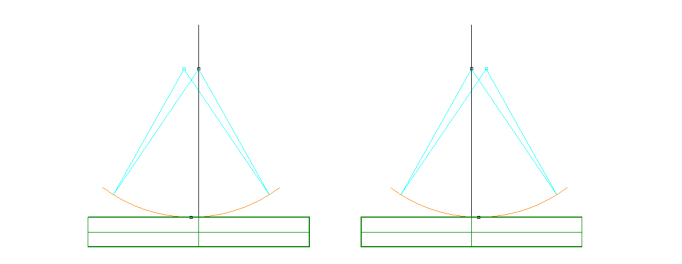
The first point to make clear is that alignment and centering are first order operations; aberrations do not make any difference. If some surface is creating an image that is too aberrated to center on or to find a best focus axial position, stop the surface down enough to get a good image. Any good optic will have a smooth, continuous surface so light reflecting from a small region of the surface is representative of the whole surface from an alignment viewpoint.
A good illustration of this is finding the vertex radius and off axis distance of an off-axis parabola. If the mirror is at all fast the image viewed at the center of curvature it will have enough coma that the two astigmatic foci are difficult to isolate definitively. By stopping down the surface the coma is reduced and the two line foci can be measured with sufficient precision that the tangential and sagittal radii can be determined. Once these are known they can be plugged into formulas for the other parameters of the segment2.
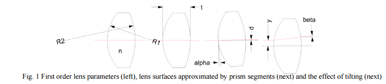
The second point is that, in terms of tilts and decenters, lenses can be thought of as wedges or prisms from a first order view point. As in Fig. 1, if a lens is decentered, the ray between object and image (an axial ray) strikes a small wedge at an angle related to the decenter and radii of the surfaces. For tilts, it is as if the ray strikes a plane parallel plate and is displaced but not changed in angle.
Assume we have a lens with radii R1 and R2, center thickness t and index n. Then the displacement of a ray along the optical axis will be d = t*α*(n-1)/n where α is the angle of incidence, that is, the tilt of the lens in this case. If a lens is decentered, the slope of the surface where a ray along the optical axis hits it will be y/R so the total wedge due to both surfaces will be γ = y*(1/R1 – 1/R2) so the deviation of the ray exiting will be β = γ*(n-1). Obviously these are small angle approximations but if the angles were large the lens wouldn’t work anyway. Also note that tilted lenses displace the ray and decentered lenses tilt, or change the angle, of the ray.
3. SIMULATION OF ALIGNMENT AND CENTERING IN A DESIGN PROGRAM
We can simulate the tilt and decenter in a lens design program using “coordinate breaks” as they are called in Zemax, or the equivalent, in other codes. As opposed to tolerancing where every surface and spacing is moved independently, once a real lens is made the front surface is physically tied to the rear surface and the lens code should reflect this fact. The code should be set up as in Table 1.
The coordinate breaks (CB) outside of the lens, lines 1 and 5, affect the whole lens and can be used to decenter or tilt it as a whole. The CB on line 1 introduces the decenter of tilt while that on line 5 removes its effect. Notice that by a judicious choice of tilt and decenter, the first surface will remain normal to a centered ray while the ray will encounter a tilted second surface. It is easier to use just the decenter without tilt and specifically introduce wedge using CB’s 1 and 3. Then it is easy to know exactly how much wedge is introduced. Furthermore, this is the way centering is specified in the ISO 10110 – Part 6 optical drawing standard3 , the wedge in the second surface relative to the first. Similarly, one could use CB’s at 3 and 5 to keep an on-axis ray normal to the first surface.
Notice that for thicknesses, the distance between the CB and surface is zero on either side of surface 1. Then the ray travels t to surface 2 where the final CB is immediately after the surface. It is important to get the spacings correct.
4. OPTICAL AXIS DEFINITION
My definition of the optical axis of a lens is one for which there are no exceptions, and that fits operationally what we are trying to accomplish, centering and alignment. The optical axis of a lens is the line joining the centers of curvature of the two surfaces. It is hard to argue with this definition and we will be doing our alignment using centers of curvature. A first apparent exception is a plano-convex or concave lens but here the axis is the line that passes through the center of curvature of the curved side and is normal to the plano side. Also, it is easy to establish a normal to the plano side with a collimated beam of light.
It is important to remember that an axis is defined by 4 degrees of freedom, either two points each defined by two degrees of freedom, or one point and one angle, each defined by two degrees of freedom. This means that when locating a lens, all 4 degrees of freedom must be constrained. Of course there is an additional degree of freedom that must be specified, the axial distance from some other datum such as a lens surface.
As a corollary to the above, note that a single spherical surface has no axis. It is defined by a point and a radius. A surface may appear to have an axis defined by the edge but this is mechanical and only defines whether a surface will be illuminated uniformly. The edge may be how the surface is mounted but does not define an optical axis.
5. CALCULATION OF CENTERS OF CURVATURE AND CONJUGATES
Now that we have settled on definitions we can get down to the heart of the matter, finding the lens conjugates. First assume we have a lens defined by R1 = 10, R2 = -6, t = 3 and n = 1.5. Assume, too, that we have a converging cone of light we are using to probe for the conjugates and that when the probe is focused on the vertex of R1 our height scale is set to 0 (see Fig. 2, top). The probe can be almost any device that has a real focus and it is helpful to have a reasonably long working distance as this gives more flexibility in terms of the ease of measuring surfaces. An autostigmatic microscope such as the Point Source Microscope is one example, but an interferometer and transmission sphere, or an alignment telescope (for centering only), could be used just as well.
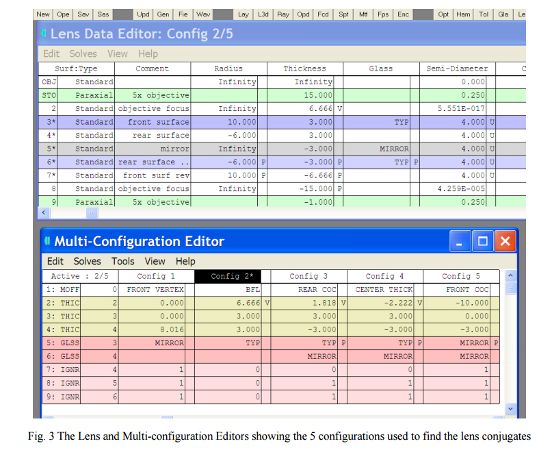
While we are doing first order, or paraxial, optics, we also want to have axial sensitivity to best focus on conjugates. This means that it is good to have a fairly fast beam of light coming from the probe. A 0.1 NA cone or somewhat faster is about right to give good sensitivity to focus. Fig. 2 shows the 5 configurations described below.
5.1 The radius of curvature of the front surface
Assuming the probe lens used to produce a point source of light has sufficient working distance, the probe is moved from being focused on the vertex of the front surface toward the center of curvature of R1 . When the focus reaches the center of curvature a spot will appear and then shrink to a minimum diameter at best focus on the center of curvature. The distance the probe moved from vertex to center of curvature is the radius of the front surface. This radius is known without any further calculation and is generally the farthest the probe has to move in the positive direction.
When focused on the vertex a Cat’s eye reflection is gotten and the return spot of light will not moved laterally as the surface, or microscope, is moved laterally. The spot may vignette and loose brightness but does not move. This is different from being focused at the center of curvature. Here, a lateral movement of the surface or microscope will cause the spot to move return laterally.
5.2 Optical center thickness
If the microscope is move toward the lens from being focused on the vertex the first return spot is usually the Cat’s eye reflection off the rear vertex and the distance moved gives the optical, t0, as opposed to the physical center thickness, t. It depends on R1, n and t. We find from paraxial optics that
As seen in the third picture in Fig. 2 the fairly steep ray going into the lens is decreased in slope so it reaches the rear vertex before the projection of the incoming ray reaches the opposite vertex. Again, this will be the usual case but can change markedly depending on the radii and glass type. Watch signs carefully while doing the calculations.
5.3 Rear surface center of curvature
For a positive lens the rear surface center of curvature will generally lie outside the lens, or on the negative side of zero the way we have defined things. Here the radius of the first surface, index and thickness as well as the rear surface radius will all affect the apparent rear surface center of curvature. As shown in Fig. 1 the rays entering the first surface are bent toward the axis so the center of curvature is closer to the first surface than the physical center of curvature.
In this case we have
where R2 is negative.
5.4 Back focal length
Calculating the back focal length is particularly useful for the case when the first surface radius is too long for the working distance of the probe being used. In this case a plane mirror is placed behind the lens being centered or investigated and a focus will be found outside the first surface vertex for a positive lens as in the lower panel of Fig. 2. If the other conjugates can be measured easily, the bfl measurement is a good cross check because as one moves along the axis, the conjugate foci are not labeled as to where they are coming from and it is easy to make a mistake. Having a way of cross checking is very useful.
For the bfl we have
You can do the first order ray trace or check reference2 for the derivation.
6. FINDING CONJUGATES USING A LENS DESIGN PROGRAM
Another way of doing what has been described above is to use a lens design code. Fig. 3 shows the five configurations above in the Multi-configuration editor in Zemax. The IGNR operand tells the program to ignore that surface for a particular configuration. The code will optimize to find the correct spacing of surface 2 to find the conjugates we are looking for on line 3 of the Multi-Configuration Editor. Remember that a finite aperture is needed to get enough rays through to optimize but a large aperture will give spacings that correct aberrations, not paraxial spacings. One way to check if the aperture is small enough is the compare the optimization value of the bfl with the General data in the prescription. The general data are paraxial calculations and will directly calculate the bfl from a paraxial ray trace.
7. DETECTING CENTERS OF CURVATURE AND CONJUGATES
Assuming now that the lens is sitting on a seat ready for centration on a rotary bearing, conjugates that are vertices will produce Cat’s eye reflections and will not move even if the lens is decentered. The Cat’s eye reflections are useful for setting crosshairs in x and y as to where a center of curvature return should appear on the video screen because the Cat’s eye falls on the optical axis of the test device or probe.
A reflection from a center of curvature will move whenever the lens is rotated on a rotary table unless the lens is perfectly centered. The center of the rotation of the spot depends on whether the microscope objective is lying on the mechanical axis of the rotary table but has nothing to do with how well centered the lens is. It is convenient to have the return from a center of curvature rotate about the center of the screen but it is not necessary. If the return spot moves the lens is not centered, or you have a rotary table with too much wobble to be useful.
Since we have said the optical axis is the line joining the centers of curvature it makes sense to center using these conjugates. Sometimes one or the other is inconvenient to reach and another such as the bfl is a better choice for one of the conjugates.
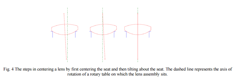
To give a general example we use the example lens from above and show how by adjusting the decenter of the lower seat and the tilt of the whole lens, the lens can be centered. As shown in Fig. 4, the rear surface sits on the seat and in general is both tilted and decentered to start with. With the probe focused on the center of curvature of the rear surface, the seat is centered until the focused spot does not move. Then the probe is moved toward the lens down to the front surface center of curvature and the lens slid in the seat until the focus spot does not move. Notice the lens is tilting around the center of curvature of the rear surface and this is why the seat must be centered first and then the lens is tilted. If it is done the other way around the process of centering diverges.
The centering should be complete in these two steps but it is best to go back and double check the upper or rear surface center of curvature to make sure nothing moved while centering the second surface. Also, if there is substantial tilt of the lens to begin with the center of curvature of the rear surface will not be physically where it appears to be optically because of refraction at the first surface. This may also call for iteration to make sure the lens is completely centered. Once both centers of curvature are stationary, or centered within the tolerance, the lens may be cemented.
7. CONCLUSION
We have pointed out that alignment and centering operations deal with the first order properties of lenses and mirrors. If aberrations interfere with obtaining good conjugate data the surfaces may be stopped down to obtain good images for alignment. Once a definition for the optical axis is given it is easy to find the conjugates for a lens, and then use these and a precision rotary table to center lenses in a cell. Following a step by step procedure it is not difficult to get centers of curvature to lie on an axis to a few micrometers TIR.
REFERENCES
[1] Optical Perspectives Group, LLC
[2] Smith, W., [Modern Optical Engineering, 3rd ed.], McGraw –Hill, New York, p. 485 and 40 (2000).
Centering with the Point Source Microscope (PSM) is a perfect application.
Centering with the Point Source Microscope (PSM) is a perfect application. When a spot of light from the objective focus is reflected back from a concave surface sitting on a rotary table, it will sweep out a circle on the video screen as the table is rotated unless the center of curvature of the surface lies precisely on the axis of rotation of the table. The picture below illustrates this.
In the picture, the point source of light lies on the axis of the rotary table but the vertex of the surface does not. The reflected spot will be twice as far away from the axis as the vertex of the surface. When the rotary table has been turned 180° as in the picture to the right, the reflected spot has moved to the other side of the axis of the table. A combination of the doubling effect of reflection and the doubling effect of a 180° rotation gives the method great sensitivity. Since a PSM can easily measure to a fraction of a μm, it is easy to center even better.
Note that the point source of light does not have to lie precisely on the axis of the table. It just has to be centered well enough that light makes it back in the objective as the table rotates. In this case, the decenter spot will still rotate but not about the center of the screen. This does not matter. If the spot rotates at all in synchronism with the rotary table the surface is not centered.
Notice, too, that the larger the diameter of the circle the spot sweeps out, the larger the decenter of the surface. Thus it is relatively easy to gradually bring a surface to better and better centration.