Conjugate Selection For Precision Lens Centering

ABSTRACT

The concept of centering a precision, symmetric lens system using a high-quality rotary table and an auto-focusing test instrument are well known. Less well known are methods of finding convenient, or easily accessible, lens conjugates on which to focus while performing the centering operation. We introduce methods of finding suitable conjugates and centering configurations that lend themselves to practical centering solutions.

1. INTRODUCTION

The act of assembling optical systems is often overlooked until the time comes to actually put the hardware together. By then thinking about the problem is too late because the customer is screaming for the system and there is no time or money to do the job correctly. The results are obvious; those responsible for the actual putting glass in cells are working overtime under great pressure and often the system produces less than optimum performance. This paper hopes to address some of the issues of assembly that can be looked at ahead of time so that some of the data needed by the assembly personnel are available when they are needed.

Another aspect of the same scenario is that Optical Perspectives makes an autostigmatic microscope, the Point Source Microscope (PSM)1 , that is useful during assembly for alignment and centering of the optical elements. As a result numerous questions are raised about how the PSM can be used during assembly, and even more comments, about why it appears to them that the PSM will be of little use. These comments generally come from the optical design people who worry about the things they see when designing lenses but have little applicability during assembly.

One reason is happens is that the design people look at perfectly aligned systems on their computer screens and have to purposefully misalign the elements to see how this affects performance. Further, if something gets so misaligned the answers do not make sense, all they have to do is hit the undo button and start over with a smaller perturbation. Another aspect of this is the way many design programs tolerance systems; they do not perturb element by element but surface by surface, something that cannot be done in practice because one surface is physically tied to a second and that has practical consequences as to what can be done to fix certain problems.

The situation is just the opposite for the assembly personnel; the elements come to them about as misaligned as they can be. One of the first things they have to do is make sure they are putting the lens in with the correct surface first. Sometimes they are given elements that are too large to fit the mounts or do not meet drawing specifications but they have no way of knowing because there was no incoming inspection. Their job is to get the assembly together quickly with no finger prints or other obvious defects and have it meet system level specifications. We want to consider some of the aspects of thinking about assembly ahead of time that will make life easier for the assembly personnel and hopefully lead to a better product.

2. ALIGNMENT AND CENTERING ARE FIRST ORDER PROPERTIES

The first point to make clear is that alignment and centering are first order operations; aberrations do not make any difference. If some surface is creating an image that is too aberrated to center on or to find a best focus axial position, stop the surface down enough to get a good image. Any good optic will have a smooth, continuous surface so light reflecting from a small region of the surface is representative of the whole surface from an alignment viewpoint.

A good illustration of this is finding the vertex radius and off axis distance of an off-axis parabola. If the mirror is at all fast the image viewed at the center of curvature it will have enough coma that the two astigmatic foci are difficult to isolate definitively. By stopping down the surface the coma is reduced and the two line foci can be measured with sufficient precision that the tangential and sagittal radii can be determined. Once these are known they can be plugged into formulas for the other parameters of the segment².

The second point is that, in terms of tilts and decenters, lenses can be thought of as wedges or prisms from a first order view point. As in Fig. 1, if a lens is decentered, the ray between object and image (an axial ray) strikes a small wedge at an angle related to the decenter and radii of the surfaces. For tilts, it is as if the ray strikes a plane parallel plate and is displaced but not changed in angle.

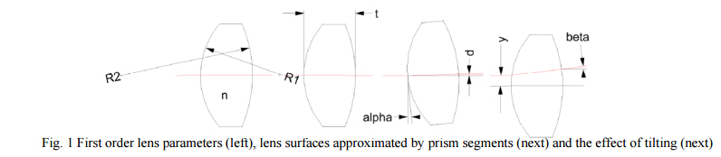
Assume we have a lens with radii R1 and R2, center thickness t and index n. Then the displacement of a ray along the optical axis will be d = t*α*(n-1)/n where α is the angle of incidence, that is, the tilt of the lens in this case. If a lens is decentered, the slope of the surface where a ray along the optical axis hits it will be y/R so the total wedge due to both surfaces will be γ = y*(1/R1 – 1/R2) so the deviation of the ray exiting will be β = γ*(n-1). Obviously these are small angle approximations but if the angles were large the lens wouldn’t work anyway. Also note that tilted lenses displace the ray and decentered lenses tilt, or change the angle, of the ray.

3. SIMULATION OF ALIGNMENT AND CENTERING IN A DESIGN PROGRAM

We can simulate the tilt and decenter in a lens design program using “coordinate breaks” as they are called in Zemax, or the equivalent, in other codes. As opposed to tolerancing where every surface and spacing is moved independently, once a real lens is made the front surface is physically tied to the rear surface and the lens code should reflect this fact. The code should be set up as in Table 1.

The coordinate breaks (CB) outside of the lens, lines 1 and 5, affect the whole lens and can be used to decenter or tilt it as a whole. The CB on line 1 introduces the decenter of tilt while that on line 5 removes its effect. Notice that by a judicious choice of tilt and decenter, the first surface will remain normal to a centered ray while the ray will encounter a tilted second surface. It is easier to use just the decenter without tilt and specifically introduce wedge using CB’s 1 and 3. Then it is easy to know exactly how much wedge is introduced. Furthermore, this is the way centering is specified in the ISO 10110 – Part 6 optical drawing standard3 , the wedge in the second surface relative to the first. Similarly, one could use CB’s at 3 and 5 to keep an on-axis ray normal to the first surface.

Notice that for thicknesses, the distance between the CB and surface is zero on either side of surface 1. Then the ray travels t to surface 2 where the final CB is immediately after the surface. It is important to get the spacings correct.

4. OPTICAL AXIS DEFINITION

My definition of the optical axis of a lens is one for which there are no exceptions, and that fits operationally what we are trying to accomplish, centering and alignment. The optical axis of a lens is the line joining the centers of curvature of the two surfaces. It is hard to argue with this definition and we will be doing our alignment using centers of curvature. A first apparent exception is a plano-convex or concave lens but here the axis is the line that passes through the center of curvature of the curved side and is normal to the plano side. Also, it is easy to establish a normal to the plano side with a collimated beam of light.

It is important to remember that an axis is defined by 4 degrees of freedom, either two points each defined by two degrees of freedom, or one point and one angle, each defined by two degrees of freedom. This means that when locating a lens, all 4 degrees of freedom must be constrained. Of course there is an additional degree of freedom that must be specified, the axial distance from some other datum such as a lens surface.

As a corollary to the above, note that a single spherical surface has no axis. It is defined by a point and a radius. A surface may appear to have an axis defined by the edge but this is mechanical and only defines whether a surface will be illuminated uniformly. The edge may be how the surface is mounted but does not define an optical axis.

5. CALCULATION OF CENTERS OF CURVATURE AND CONJUGATES

Now that we have settled on definitions we can get down to the heart of the matter, finding the lens conjugates. First assume we have a lens defined by R1 = 10, R2 = -6, t = 3 and n = 1.5. Assume, too, that we have a converging cone of light we are using to probe for the conjugates and that when the probe is focused on the vertex of R1 our height scale is set to 0 (see Fig. 2, top). The probe can be almost any device that has a real focus and it is helpful to have a reasonably long working distance as this gives more flexibility in terms of the ease of measuring surfaces. An autostigmatic microscope such as the Point Source Microscope is one example, but an interferometer and transmission sphere, or an alignment telescope (for centering only), could be used just as well.

While we are doing first order, or paraxial, optics, we also want to have axial sensitivity to best focus on conjugates. This means that it is good to have a fairly fast beam of light coming from the probe. A 0.1 NA cone or somewhat faster is about right to give good sensitivity to focus. Fig. 2 shows the 5 configurations described below.

5.1 The radius of curvature of the front surface

Assuming the probe lens used to produce a point source of light has sufficient working distance, the probe is moved from being focused on the vertex of the front surface toward the center of curvature of R1 . When the focus reaches the center of curvature a spot will appear and then shrink to a minimum diameter at best focus on the center of curvature. The distance the probe moved from vertex to center of curvature is the radius of the front surface. This radius is known without any further calculation and is generally the farthest the probe has to move in the positive direction.

When focused on the vertex a Cat’s eye reflection is gotten and the return spot of light will not moved laterally as the surface, or microscope, is moved laterally. The spot may vignette and loose brightness but does not move. This is different from being focused at the center of curvature. Here, a lateral movement of the surface or microscope will cause the spot to move return laterally.

5.2 Optical center thickness

If the microscope is move toward the lens from being focused on the vertex the first return spot is usually the Cat’s eye reflection off the rear vertex and the distance moved gives the optical, t0, as opposed to the physical center thickness, t. It depends on R1, n and t. We find from paraxial optics that

As seen in the third picture in Fig. 2 the fairly steep ray going into the lens is decreased in slope so it reaches the rear vertex before the projection of the incoming ray reaches the opposite vertex. Again, this will be the usual case but can change markedly depending on the radii and glass type. Watch signs carefully while doing the calculations.

5.3 Rear surface center of curvature

For a positive lens the rear surface center of curvature will generally lie outside the lens, or on the negative side of zero the way we have defined things. Here the radius of the first surface, index and thickness as well as the rear surface radius will all affect the apparent rear surface center of curvature. As shown in Fig. 1 the rays entering the first surface are bent toward the axis so the center of curvature is closer to the first surface than the physical center of curvature.

In this case we have

where R2 is negative.

5.4 Back focal length

Calculating the back focal length is particularly useful for the case when the first surface radius is too long for the working distance of the probe being used. In this case a plane mirror is placed behind the lens being centered or investigated and a focus will be found outside the first surface vertex for a positive lens as in the lower panel of Fig. 2. If the other conjugates can be measured easily, the bfl measurement is a good cross check because as one moves along the axis, the conjugate foci are not labeled as to where they are coming from and it is easy to make a mistake. Having a way of cross checking is very useful.

For the bfl we have

You can do the first order ray trace or check reference² for the derivation.

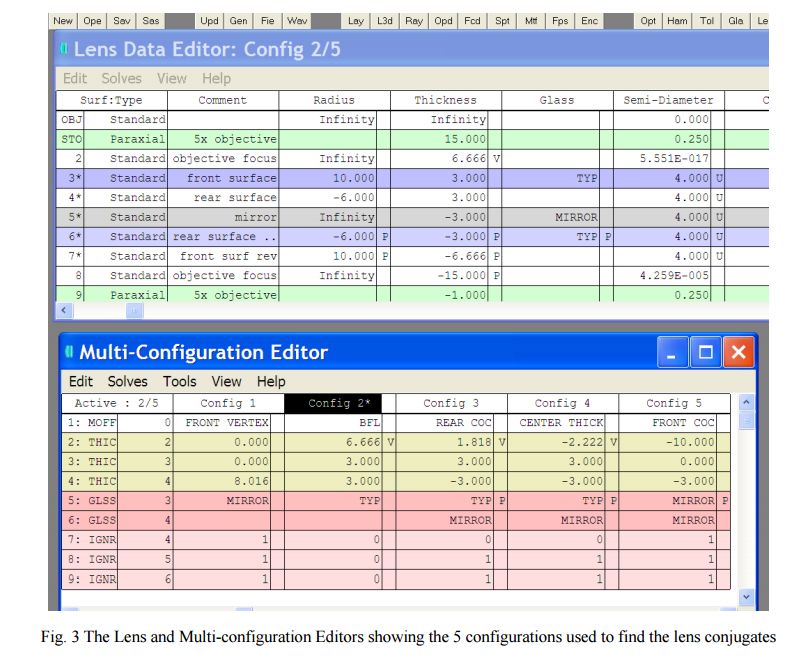
6. FINDING CONJUGATES USING A LENS DESIGN PROGRAM

Another way of doing what has been described above is to use a lens design code. Fig. 3 shows the five configurations above in the Multi-configuration editor in Zemax. The IGNR operand tells the program to ignore that surface for a particular configuration. The code will optimize to find the correct spacing of surface 2 to find the conjugates we are looking for on line 3 of the Multi-Configuration Editor. Remember that a finite aperture is needed to get enough rays through to optimize but a large aperture will give spacings that correct aberrations, not paraxial spacings. One way to check if the aperture is small enough is the compare the optimization value of the bfl with the General data in the prescription. The general data are paraxial calculations and will directly calculate the bfl from a paraxial ray trace.

7. DETECTING CENTERS OF CURVATURE AND CONJUGATES

Assuming now that the lens is sitting on a seat ready for centration on a rotary bearing, conjugates that are vertices will produce Cat’s eye reflections and will not move even if the lens is decentered. The Cat’s eye reflections are useful for setting crosshairs in x and y as to where a center of curvature return should appear on the video screen because the Cat’s eye falls on the optical axis of the test device or probe.

A reflection from a center of curvature will move whenever the lens is rotated on a rotary table unless the lens is perfectly centered. The center of the rotation of the spot depends on whether the microscope objective is lying on the mechanical axis of the rotary table but has nothing to do with how well centered the lens is. It is convenient to have the return from a center of curvature rotate about the center of the screen but it is not necessary. If the return spot moves the lens is not centered, or you have a rotary table with too much wobble to be useful.

Since we have said the optical axis is the line joining the centers of curvature it makes sense to center using these conjugates. Sometimes one or the other is inconvenient to reach and another such as the bfl is a better choice for one of the conjugates.

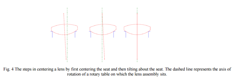
To give a general example we use the example lens from above and show how by adjusting the decenter of the lower seat and the tilt of the whole lens, the lens can be centered. As shown in Fig. 4, the rear surface sits on the seat and in general is both tilted and decentered to start with. With the probe focused on the center of curvature of the rear surface, the seat is centered until the focused spot does not move. Then the probe is moved toward the lens down to the front surface center of curvature and the lens slid in the seat until the focus spot does not move. Notice the lens is tilting around the center of curvature of the rear surface and this is why the seat must be centered first and then the lens is tilted. If it is done the other way around the process of centering diverges.

The centering should be complete in these two steps but it is best to go back and double check the upper or rear surface center of curvature to make sure nothing moved while centering the second surface. Also, if there is substantial tilt of the lens to begin with the center of curvature of the rear surface will not be physically where it appears to be optically because of refraction at the first surface. This may also call for iteration to make sure the lens is completely centered. Once both centers of curvature are stationary, or centered within the tolerance, the lens may be cemented.

7. CONCLUSION

We have pointed out that alignment and centering operations deal with the first order properties of lenses and mirrors. If aberrations interfere with obtaining good conjugate data the surfaces may be stopped down to obtain good images for alignment. Once a definition for the optical axis is given it is easy to find the conjugates for a lens, and then use these and a precision rotary table to center lenses in a cell. Following a step by step procedure it is not difficult to get centers of curvature to lie on an axis to a few micrometers TIR.

REFERENCES

[1] Optical Perspectives Group, LLC

[2] Smith, W., [Modern Optical Engineering, 3rd ed.], McGraw –Hill, New York, p. 485 and 40 (2000).

[3] Available from http://webstore.ansi.org/