Customers purchasing a PSM often ask me if we offer mounting hardware for the PSM like x-y-z stages.
MY ANSWER HAS BEEN “NO”, BECAUSE THERE ARE SO MANY WAYS OF USING THE PSM THAT IT WOULD BE IMPOSSIBLE TO MEET EVERYONE’S DIFFERENT NEEDS.
IN FACT, THE ANSWER IS “YES!”
The centering station is a tall, motorized and encoded z stage with x-y lateral adjustments more than adequate to keep an image within the PSM field of view.
I use the centering station daily because it is so convenient.
Rather than attaching the PSM to an x-y-z mount as a first step, I simply move the lens or assembly to the centering station and I am ready for almost any type of lens measurement.
For any sort of measurement you might do on a classical optical bench, the centering station is a convenient and cost effective solution.
The MicroFinish Topographer helped bring you this spectacular image of the sun.
The smoothness criterion on the Daniel K. Inouye Solar Telescope primary mirror was a scatter specification. This was a problem in two respects, the mirror substrate was Zerodur and the scatter angle was too close to specular to measure with a scatterometer. The near zero expansion Zerodur is a microcrystalline glass ceramic that scatters light when illuminated so a scatter test could not be used during polishing. Also, the scatter angle in the specification was so close to specular that the detector in a scatterometer partially obscured the scattered light path and could not be used even if the substrate did not scatter.
Kashmira Tayabala, et. al., “Use of the PSD and incident angle adjustments to investigate near specular scatter from smooth surfaces”, Proc. SPIE, 8838 (2013) showed that the MicroFinish Topographer (MFT) could measure surface roughness over sufficiently long distances to infer the magnitude of the near specular angle scatter. Given this insight, the MFT was used to show the Inouye Solar Telescope primary met the near specular angle scatter specification, Chang Jin Oh, et. al., “Fabrication and Testing of 4.2m Off-Axis Aspheric Primary Mirror of Daniel K. Inouye Solar Telescope”, Proc. SPIE, 9912 (2016).
A combination of the Auto Gain function of the Point Source Microscope (PSM) and the use of an Axicon grating make centering of severely misaligned lenses easy.
The lenses in the cell are misaligned far enough that light in the center of the aperture barely makes it through the lens.
The PSM video screen displays a partial set of rings produced by a combination of the PSM and Axicon grating. The orientation and curvature of the rings indicates how the lens cell must move to center it with respect to the Axicon grating axis. Note that the PSM objective focus is at an arbitrary height about the lenses, not at a back focus, or center of curvature of one of the lens elements
The first video picture (left) shows the partial ring pattern with the lens misaligned as in the picture above. As the lens is moved by the screws it is clear the centering gets better (middle). The next picture (right) shows the center of the Axicon grating pattern now in the field of view of the video screen. The magenta crosshair is barely visible in the center of all three pictures and is the reference for centering.
The bright spot in the center of the Axicon grating pattern is much more intense than any of the rings. This intensity forces the Auto Gain function to reduce the gain and shutter exposure time so there are no saturated pixels in the display so the final centered pattern looks like the picture on the left side above where only the center spot and first few rings are visible centered on the crosshair. The picture on the right is a blow up of the one on the left to make the crosshair and scale bar easier to see.
The full screen shot shows that the central spot is centered to less than 1 μm. Also, the Auto Gain was turned off so that more detail in the rings is visible.
The centering was accomplished as fast as the adjustment screws could be turned. This contrasts with the conventional situation where the centering objective must first adjusted to focus at a back focus or center of curvature so there is sufficient focused intensity to view on the video screen. Then the lens cell is moved around to find the focused spot that is lying outside the field of view of the microscope. This is often the most difficult part of the alignment, finding the focused spot when there is no signal on the detector until you are within the field of view of the objective, typically within 0.5 mm when using a 10x objective.
With the Axicon grating the alignment is much faster than conventional methods and less tedious because there is a useful centering indicator even though the lens system is vastly decentered. The lack of tedium makes the work of centering pleasurable rather than a chore.
Recently a customer was using the Point Source Microscope (PSM) to align a slow, singlet objective lens and find its focus.
The customer had a plane retro mirror behind the objective and should have seen a nice round spot at best focus. Instead, he saw a vertical line image as in the following screen shot of the PSM computer display.
The customer knew the PSM was working correctly because he did get a small, round image when he focused at the center of a good grade steel ball. He also knew the lens was correctly aligned to the PSM because he had used the PSM in the autocollimator mode and had reflections from both sides of the lens centered on the PSM electronic crosshairs.
When he did decenter the PSM and looked at the reflected image on a white card he saw a line image. In addition, when he tried to refocus over a 25 mm range he could not find a circle of least confusion. All this pointed to a severely astigmatic return wavefront since the lens was from a trusted vendor. The test set up is shown in the picture below. The rear of the PSM is in the foreground and the objective is at the far end of the optical table with an undersized plane mirror behind it.
I suggested that it might be the small, plane retro return mirror was not flat because the mount was squeezing it. He assumed this was not the case but said he would check.
Not long after I got an email with this picture showing the great improvement in the image after remounting the return mirror.
Clearly, the problem is not completely solved, but the image is many times better than before and the source of the problem isolated. The PSM laser diode source is in the maximum intensity mode that makes the image larger than it should be due to saturated pixels in the camera, and there is still some astigmatism in the wavefront or the spot would be round. The red line just under the horizontal line image is 100 μm long for scale. The lens was about 2 m from the PSM so the roughly 250 μm long image has an angular width of about 5 seconds of arc. The height of the image is slightly more than one would expect due to diffraction.
This is just one example of how the PSM can spot a problem in a test set up before the problem becomes serious. The problem might be serious due to the time it takes to track down its source, or if the problem is not fixed, the issues it will create farther downstream if not corrected at the source.
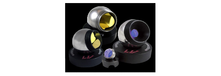
Spherically mounted retroreflectors (SMRs) are an essential part of spatial metrology when using a laser tracker. However, the precision of the laser tracker measurement is no better than the precision with which the cube corner retroreflector is mounted in the spherical ball. Thus measuring the position of the apex of the cube corner with respect to the center of the ball is a critical part of both the assembly and inspection of SMRs. This leads to cost implications because the better centered the cube corner in the ball, the more the SMR costs.
We begin by explaining the use of SMRs with a laser tracker, and then explain how the question arose of whether an autostigmatic is useful in measuring the apex location of the cube corner. We follow this with the theory of the measurement based on a two-dimensional argument, but the same argument applies to the three-dimensional case. The two-dimensional case is much easier to explain and understand.
Finally, we look at how real hardware must be fixtured to make the measurements. At first it looks difficult because a sphere has no axis and the SMR must rotate about orthogonal axes to measure the apex location. However, a very simple fixture is satisfactory. We give some measured results to demonstrate the precision of the method.
2. USING SMRS
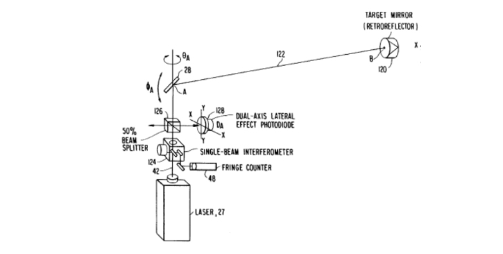
Fig. 1 is from US Patent 4,714,339 that describes a laser tracker. Light from a laser projects from a measuring head that rotates in azimuth and elevation. The light reflects back to the tracker from a target that is a cube corner retroreflector. There is a position-tracking sensor built into the head so the motorized azimuth and elevation axes follow the target and encoders on the axes record the angles versus a time base. In addition, there is a time of flight sensor that measures the distance to the target completely specifying the target position in a spherical coordinate system centered about the intersection of the azimuth and elevation axes of the head.
The cube corner retroreflector target mounts in a hollow ball such that its apex ideally sits at the center of the ball. The laser tracker metrology field calls this arrangement of a cube corner in a ball a spherically mounted retroreflector, or SMR. The SMR sits in a kinematic nest1 attached to the structure being measured as shown in Fig. 2. The precision nest allows precise positioning to datums on the structure. Assuming a precise positioning of the nest, the SMR contributes an error to the measurement of twice the displacement of the apex to the center of the ball in all 3 degrees of translational freedom. Since laser trackers are capable of measurements in the range of a few μm’s and a few seconds of arc2,3,4, the errors in the SMR contribute directly to the total error of the measurement.
3. PRECISE POSITIONING OF LASER TRACKER NESTS
Before discussing how we got into the measurement of the cube corner SMR, we should discuss the precise positioning of the SMR nests relative to datums on the structure the laser tracker interrogates. Because the SMR ball sits in the nest and balls are very easy to align precisely with an autostigmatic microscope (ASM)5, an ASM is an ideal method to help position nests. In all the cases we show in this paper, the ASM used was a Point Source Microscope (PSM)6, a convenient, modern version of a classic ASM.
Fig. 1. Diagram of a laser tracker from US Patent 4,714,339
Fig. 2. Examples of SMRs sitting in kinematically defined, precision “nests”
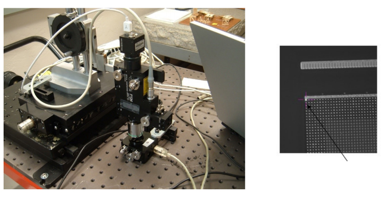
In one case, the test engineers wanted to know the location of a CCD camera image plane using a laser tracker since there was no convenient way to get to the camera during the actual test. A solution was attaching 3 nests to the exterior of the camera and using the PSM mounted on a precision stage to relate the nests, hence SMRs, to the image plane.
SMR balls come in standard sizes, one of which is 1⁄2”. By substituting full 1⁄2” balls for 1⁄2” SMRs it was simple to find the x,y,z positions of the centers of the 3 balls with the PSM. Then using the video mode of the PSM, the corners of the CCD array were located in the same coordinate system since the video image plane in the PSM is parfocal with the point source at the objective focus as in Fig. 3. This procedure tied the corners of the image plane to the 3 ball centers so that when SMRs were substituted for the solid balls, the laser tracker located the position of the CCD image plane. This is just one example of the use of the PSM to position SMR nests on the structure the laser tracker measures.
4. ORIGIN OF THE IDEA OF USING THE PSM TO MEASURE SMRS
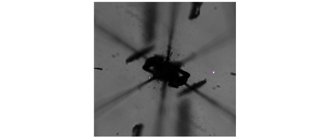
I was exhibiting the PSM at a trade show 2 years ago when a follow exhibitor came over and asked if the PSM could be used to locate the vertex of the cube corner relative to the center of the ball that held the cube corner. I had to admit I had never used the PSM to look into any kind of cube corner and did not know if the PSM would be useful. However, the question intrigued me and I set about looking for an answer. At first, it was not obvious whether the PSM should be used with a focused or collimated beam but since an objective was already installed that was tried first. When the microscope was focused down to the plane of the apex, a return reflection appeared mirrored across the apex from when the focused spot was incident. It was easy to see where the spot focused because the surfaces of the cube corner were illuminated with the LED source in the PSM while the point source was simultaneously illuminated as seen in Fig. 4.
Note that you cannot look right at the apex because it is not optically perfect and tends to collect contamination. This forces you to view the prism decentered from the apex. Then you to think the measurement cannot be made until you realize the corner reflector acts like a right angle prism and this behavior is exactly what you would expect in 2 dimensions. Now that it is clear some sort of measurement is possible, it is time to look at where the light rays are going.
Fig. 3. CCD camera with SMR nest attached to the camera body while the PSM is focused on the CCD array (right)
Fig. 4 Magnified image of the apex of a corner reflector with the PSM focus to the left of the apex and reflected spot to the right. The 6 pie segments of the reflector are obvious and as are contamination spots reflected across the apex.
5. IMAGING ON A SURFACE WITH A POINT SOURCE OF LIGHT
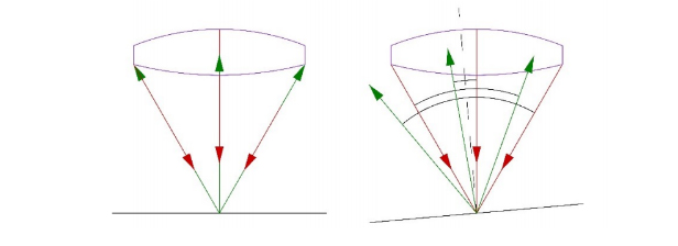
When a point source of light is imaged on a surface, we get a Cat’s eye, or retro, reflection as shown in Fig. 5. The rays incident (red) on the surface are reflected back (green) into the objective, obeying the part of the Fresnel law of reflection that says the angle of incidence equals the angle of reflection relative to the normal to the surface.
Fig. 5. A point source of light focused on a surface perpendicular and tilted with respect to the gut ray
As implied by the left picture, for every incident ray there is a reflected ray mirrored about the gut ray tracing the exact same path back into the objective lens of the microscope. The same holds when the surface tips with respect to the gut ray and center of the objective. Every incident ray reflects back into the objective mirrored about the normal to the surface, the black dotted line. The right hand picture makes it clear that not all the reflected rays make it back into the objective, nor is the surface uniformly illuminated about the normal so the reflected image appears oval, or football shaped, when viewed out of focus. The reflected spot appears round at exact best focus independent of tip.
The more important aspect of the tipped surface reflection is that the plane wave incident on the objective that creates the focused spot on the surface is parallel to the plane wave on reflection collimated by the objective. Fig. 5 implies this but it is not as obvious as the vignetting mentioned above. If a plane wave focused by an objective produces a spot at a specific location on a surface, then a point source of light in the same location on the surface projected toward the objective must produce a plane wave, once collimated by the objective, that parallels the plane wave originally producing the spot.
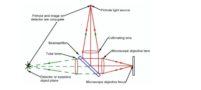
This property of the Cat’s eye, or retro, reflection is so obvious that we tend to overlook the implications, yet this is why an autostigmatic microscope is such a useful tool for aligning optics. We align the crosshair in the detector to the point source providing illumination to the surface through the objective by centroiding on the Cat’s eye reflection. The crosshair on the detector is then conjugate to the originating point source of light and to the focused spot on the surface as shown in Fig. 6.
Fig. 6. PSM ray diagram showing that the point source, its image at focus and its image on the detector are conjugate
The Cat’s eye image properties also include that the surface does not have to be plane or smooth. It is easy to obtain a Cat’s eye image off a ball or any spherical surface. At first, this seems counterintuitive but the focused sport is so small there is almost no change in the slope of the surface over the size of the spot so it behaves like a plane surface. While the best focused Cat’s eye images, in terms of a tightly focused spot, come from smooth or specular surfaces, it is easy to get a Cat’s eye from a piece of paper, for example. The spot will be larger in diameter than from a smooth surface, may be somewhat irregular in shape and will require greater source intensity to see, but will produce a spot with a minimum diameter at best focus that is conjugate to the point source of illumination.
We complete this analysis of the behavior of Cat’s eye images by going back to some geometrical definitions. Since one can pass a plane though a point it should come as no surprise that the plane can tilt around the point. Similarly, a spherical or cylindrical surface can pass through a point independent of the radius of either. These are the fundamental reasons for the behavior of a Cat’s eye image. All these properties are useful during initial alignment of test setups to get the various components roughly aligned and light back into the microscope objective for electronic video viewing.
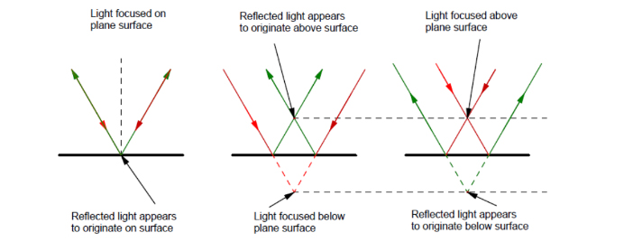
6. AXIAL BEHAVIOR OF THE CAT’S EYE REFLECTION
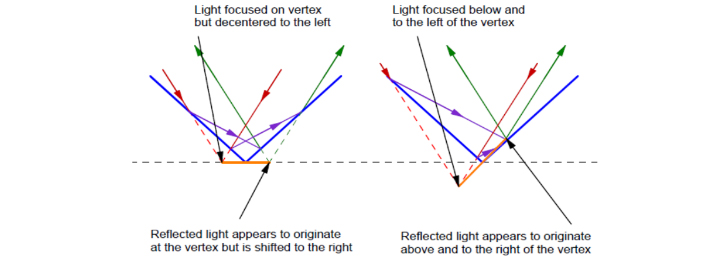
When the incident, focused spot is either above or below the surface when looking for a Cat’s eye image, the reflected spot looks like it is coming from below or above the surface, respectively, as seen in Fig. 6.
Fig. 6. Light focused above or below a surface appears mirrored in the surface axially
The incident (red) rays form a virtual focused image below the surface that produces a real reflected (green rays) image above the surface and vice versa. The dotted red and green rays are virtual.
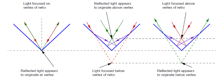
Fig. 7 shows the situation similar to Fig. 6 but this time looking into a hollow right angle reflector. This is a little harder to follow because of the extra bounce of light in the reflection but the net effect is the same as in the plane surface case, light focused below the apex looks like it is coming from above the apex, and vice versa. To make Fig. 7 a little easier to interpret the incident light is still red and the reflected green but the first reflection of the ray shows in violet. The horizontal dotted black lines show the distances above and below the apex while the colored dotted lines show the virtual rays.
Fig. 7. Light focused above or below a right angle reflector appears mirrored in the surface axially
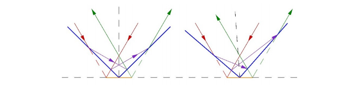
If the incident, focused spot is left or right of the apex but the same depth as the apex we have the situation in Fig. 8. This is different from a plane mirror that has no feature to create a symmetry. The apex of the hollow right angle reflector creates an axis of symmetry so that light incident to the left of the apex reflects the same distance from the apex to the right. The orange line shows the distance and orientation of the shift from the incident to the reflected virtual focus in the case (left) where the incident focus is the same depth as the apex. The situation gets more complex when the incident spot shifts laterally and axially. Again, the orange line shows the vector between the incident, and the reflected, virtual focus. The hollow reflector acts like a plane mirror to axial shifts but now has a symmetrical, lateral shift due to the axis created by the apex.
Fig. 8. Reflection from a right angle reflector where the focused incident light is not centered on the axis of the reflector (left) and not centered nor the same depth (right)
On the other hand, the hollow reflector behaves as expected when tipped about its apex and the incident light focuses at the same depth as the vertex. The lateral shift of the reflected spot does not change with tip of the reflector as seen in Fig. 9. This behavior suggests a method of finding the decenter of the apex. If the reflector turns 180 degrees but the apex is not on the axis of rotation then to the incident light the apex appears closer in one orientation than the other does. This means the reflected spot appears to move by twice the decenter of the axis of rotation from the apex.
Fig. 9. Reflection from a right angle reflector when the reflector angle bisector is parallel to the objective gut ray (right), or the reflector is tipped relative to the gut ray. (The tilt is slight so the Figure does not get too complex.)
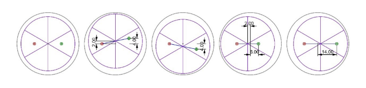
7. MEASUREMENT OF APEX DECENTER
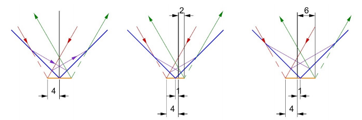
In Fig. 10, we show that if the reflector is rotated about an axis decentered 1 unit from the apex, the reflected spot moves 4 units laterally. In the picture on the left, the axis of rotation (heavy black line) is centered on the reflector apex and the incident focused spot is 4 units to the left is the apex. In the middle picture, the apex shifts 1 unit to the left of the axis of rotation but the spot is still 4 units from the axis of rotation. After rotating the reflector 180 degrees as in the right picture, the spot is still focused 4 units from the axis of rotation. Comparing the middle and right hand pictures, we see that the reflected spot moves from 2 units relative to the axis of rotation to 6 units upon rotation, or a 4x movement of the apex from the axis of rotation.
Fig. 10. Light incident 4 units from the apex (left), the reflector shifted 1 unit to the left (middle) and shifted 1 unit to the right by virtue of a 180° rotation about an axis 4 units from the incident spot.
We drew Fig. 10 using a CAD program to trace the rays but if you used algebra and trigonometry you would come to the same conclusion, as long as the incident spot is fixed relative to the axis of rotation, the reflected spot moves 4 times the decenter of the apex relative to axis of rotation. This is because the reflected spot is always symmetric with the incident spot about the apex. Because the apex shifts toward the incident spot in the middle picture, the reflected spot moves twice as much to the left. The opposite happens when the reflector is rotated 180 degrees.
8. BEHAVIOR WITH APEX ABOVE OR BELOW CENTER OF ROTATION
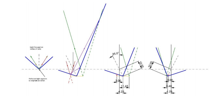
In order to find the distance between the apex of the reflector and the center of the ball, the SMR is rotated about the ball center. To get the maximum sensitivity the ball is tipped as far as possible without vignetting the beam, about 25- 30 degrees. It is difficult to draw a picture that clearly shows the true situation but Fig. 11 attempts to do so. If the beam focuses right at the apex the beam comes back upon it self. If the apex is below, or above, the center of the ball we have the case illustrated in Fig. 7 but the PSM precision is limited in the axial direction. If the ball is tilted about its center, the apex moves off the center of rotation so we have a situation somewhat like the decentered apex, and the reflected spot will shift laterally, a direction where the PSM has great sensitivity.
Fig. 11. Behavior of the reflected spot when the apex is below the center of rotation (3rd diagram) and after 180° rotation. The red and green dotted lines indicate the positions of the virtual images.
As seen in Fig. 7, if the PSM is not focused to the depth of the apex, the reflected spot will also be defocused. It is best practice to find best focus and then tip the SMR as far as possible without vignetting. Then we have the situation in the second picture of Fig. 11 where we have had to extend the reflector surface to show where the reflected ray is incident on the surface. This picture shows the overall ray paths and the bisector of the reflector faces. The bisector rotates about the ball center, the horizontal dotted line. The incident focused beam appears to reflect on the other side of the prism apex but at approximately the depth of the apex because this is where we focused the microscope.
The third and 4th pictures show more detail about the distances of the incident light and the apex that comes in at a fixed distance of 3 units from the center of the ball, or point of rotation. The apex shifts 4.23 units because this is 10*sin 25°. It is 7.235 units from the apex to the incident focus so the reflected focus is 7.235 units beyond the apex or 11.45 – 4.235. In the fourth picture, the ball was rotated 180° about a normal to the plane of incidence which moves the apex to the other side of the axis of rotation, in fact, beyond the incident focus. The reflected spot is still the same distance on the other side of the apex, 1.23 units on either side. Thus the reflected spot has moved 11.45 + 5.46 = 16.91 units, or 4 times the 4.23 unit distance the apex is from the axis of rotation. The height error, or distance from ball center to apex is 16.91/(4*sin25°) = 10.
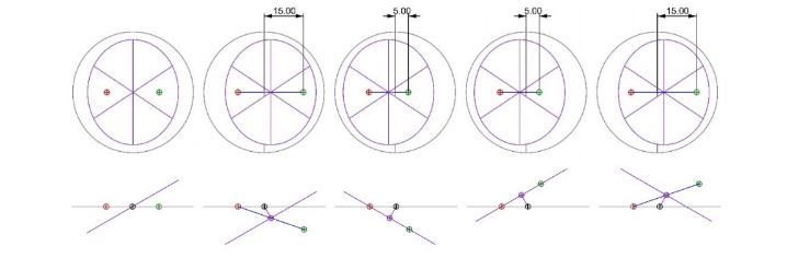
This is easier to see in Fig. 12 and 13 that summarize the decenter and height error cases. In Fig. 12 we look at a top view of the SMR, first, fully centered, then decentered 2 units up, then 2 units down. The 4th and 5th are decented 2 units left and right, respectively. In each case a line is drawn between the incident focus and the apex, and then continued on an equal distance beyond the apex to show the location of the reflected spot.
Fig. 12 Top view of SMR with incident (red) and reflected (green) spot positions as the cube corner is decentered within the ball
It is easy to see that a 2 unit decenter produces an 8 unit change in the reflected spot position upon a 180° rotation of the ball about an axis normal to Fig. 12. In reality, the motions in Fig. 12 are grossly exaggerated to show that effects of decenter. In practice, the decenters are a few tens of μm or less in commercial SMRs but the behavior of the reflected spot is the same as is shown.
Fig. 13 is a diagram showing the situation for the apex being above or below the point of rotation looking from the top and side. We have shown how to calculate the distance above or below, but we need to know if the apex above or below the point of rotation for proper correction of the error. In the left hand view in Fig. 13 the SMR tips to the left but the apex (purple dot) lies on the center of rotation (black dot) so there is no motion of the apex and no displacement of the reflected spot (green). Also notice the distance between the incident spot and center of rotation is the same in all cases, only the reflected spot moves when the apex is not on the center of rotation.
Fig. 13. Top and side views where the apex is below and above the center of rotation when the SMR tips left or right.
In the second to left picture, the apex (purple dot) of the SMR lies below the axis of rotation (black) so the apex moves to the right as the SMR tips to the left, and vice versa in the middle picture. In fact, we do not tip left and right, but rotate the SMR 180° about the normal to the aperture of the cube corner, which has the same effect as tipping to the right. When the SMR rotates 180° the reflected spot moves to the left. If the apex is above the axis of rotation, as in the right hand two pictures, the reverse is true. Relative to the initial position of the reflected spot, the reflected spot moves right when the SMR is rotated 180°.
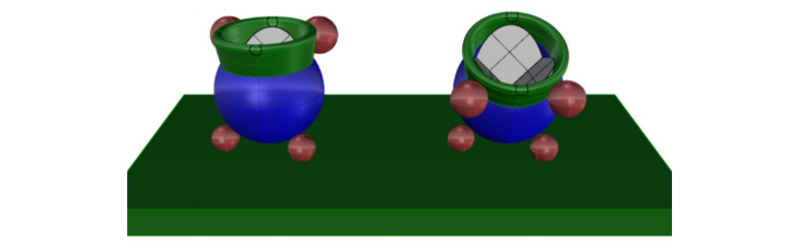
9. FIXTURE FOR MEASURING APEX LOCATION ERROR
Measuring the reflector apex location relative to the ball center requires two measurements of the reflected spot position with the reflector bisector vertical and two measurements while the reflector tilts as much as possible without vignetting, typically about 25°. With the reflector vertical, measure at an azimuth angle of 0 and 180°. Start the measurement as shown in Fig. 12, in the middle of one of the six pie shaped segments. This way the seam, or edge, of the segment does not block the beam by falling into the crack. The starting position is unimportant to the measurement because it only requires the difference in the two readings. However, if the cube corner needs centering, the direction of the decenter is important so the 0° reading should reference a feature on the SMR such as a logo or serial number.
For the height measurement, the ball tilts about 25° and the spot position is measured. The ball is rotated 180° and the measurement repeated. Again, it is a difference measurement so the starting point is irrelevant. Even the precision of the 180° rotation is not critical because an error in this angle leads to a cosine error. Only gross errors in azimuth angle are significant. Fig. 14 shows a fixture that gives repeated proper orientation to typical SMRs.
Fig. 14. A fixture with the necessary features to perform apex location measurements. The Figure shows separate features for the two measurements required for clarity but the features easily combine into one fixture.
Three balls under the SMR locate the ball center precisely while two balls behind the collar (left) on the SMR hold the ball upright. The small black circles on the collar help orient the SMR during the 180° rotation. On the right, the two balls in front of the collar control the 25° tilt and the small circles help with the 180° rotation. The Figure shows the fixture as two fixtures for clarity but obviously, the two sets of two balls could combine into one fixture.
10. EXPERIMENTAL DATA
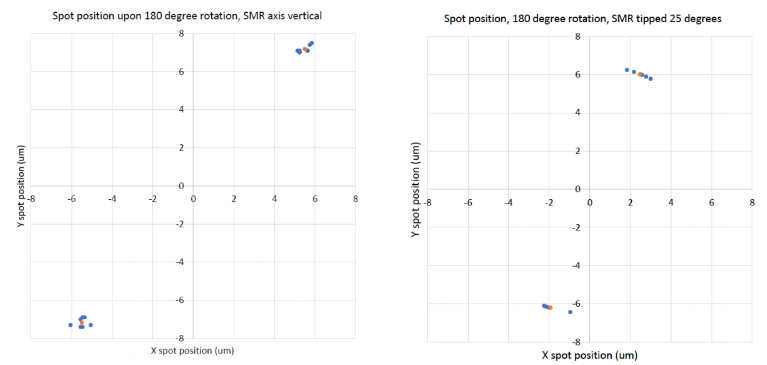
We tested a commercially available SMR sold as a standard quality SMR for reflector apex position using the methods outlined above. The standard quality designation means the apex lies within a sphere of radius 0.0005” (12.7 μm) of the center of the ball. Six measurements were made using the engraved logo as the azimuthal reference for 0 degrees and then at 180 degrees. The left chart in Fig. 15 shows the data with the orange spot being the average in the two locations. The x, y average coordinates were 5.50, 7.18 and -5.50, -7.18 μm for a spot separation of 18.09 μm at an angle of 52.6°. Since the sensitivity of the measurement is 4 times the spot separation due to the 180° rotation and doubling on reflection, the apex is 4.5 μm from the ball center at an angle of 142.6° relative to the serial number that was at the negative end of the y axis in the test setup. For decenter, this SMR meets the 0,0005” specification.
Fig. 15 Measured spot position data with the SMR vertical (left) and tipped the the right by 25° (right)
When we tipped the SMR -25° about the y axis, as opposed to Fig. 14 showing the fixture with the tip about the x axis, and repeated the measurement to get the data in the graph on the right. The average locations of the spots were 2.47, 6.01 and -1.93, -6.20 for a separation of 12.98 μm. Since the sensitivity of the measurement is increased by the sin of the angle of tip, the actual height difference between the apex and ball center is 12.98/(4*sin(25)) = 7.68 μm. Comparison of the two charts shows that when the SMR was tilted a -25° about the y axis, the x error became less indicating the apex is below the ball center. Notice the data in the y direction remains nearly the same whether the ball is tipped or not.
There are subtleties to the measurement that are not obvious at first. For one, the data shown are after subtracting the average reflected spot position because the actual distance of the incident light from the apex is completely arbitrary. What is significant is the difference between the 0° and 180 ° readings and their azimuthal angle relative to some azimuthal feature on the SMR. The arbitrariness is very useful in that it allows flexibility to avoid contamination on the corner reflector from affecting the measurement.
Also, the height and decenter measurements are coupled since tipping the SMR moves the apex laterally if the apex is above or below the ball center. This is why we measure the decenter with the reflector axis vertical, to avoid coupling in the height error. When the SMR tilts about, say, the x axis, the lateral positon of the x decenter does not change but the y decenter does if the apex is above or below the ball center. The direction of this change with tipping indicates whether the apex is high or low.
The advantages of the measurement method are clear. The test uses the simplest sort of fixture and the sensitivity of the measurement is well above the specification of the highest quality SMRs. Four data points are all that are needed to completely specify the location of the reflector apex relative to the center of the ball. It is easy to make the 4 measurements using the fixture and a suitable autostigmatic microscope in under 1 minute per SMR. Obviously repeated measurements should be made to assure a level of repeatability to meet quality assurance standards.
Since SMRs are used in many orientations, the risk of the SMR falling and being damaged is high. If the SMR is obviously broken there is only one solution; replace the SMR. On the other hand, the SMR may not show any sign of damage but the retro-reflector may have moved. This measurement technique is a quick check on possible damage.
11. CONCLUSION
We have shown how to measure the distance, in all three directions, of the apex of a spherically mounted retroreflector (SMR) relative to the center of the ball in which it is mounted. The measuring technique is simple, requires a simple fixture and is about 10 times as precise as industry standards.
12. ACKNOWLEDGEMENT
I would to acknowledge John Casstevens, of Dallas Optical Systems, Inc., for recognizing the possibility that the PSM might be applicable to measuring the location of the apex in an SMR, and for introducing the idea to Joe Gleason of Baltec, who subsequently stopped by to see if he could interest me into making the measurement. I would also like to acknowledge Robert Bridges of FARO Technologies, Inc. for providing SMRs to make additional measurements.