Author: csadmin

There was more interest in Chapter 3 about the classical instruments used for optical alignment than any other chapter to date, and I didn’t have a chance to say all I wanted to, so I will continue the discussion in this Chapter to emphasize how changes in technology have changed the design of these instruments. The instruments discussed previously are basically the same; they increase the angular sensitivity of the eye from about 1 minute of arc to something substantially greater by using two lenses of different focal lengths to increase the magnification of the eye.

The objective and eyepiece in a telescope change the angular extent of a distant object into an image that subtends a much larger angle as the nearly collimated light enters the eye from the eyepiece. A microscope is nothing more than a telescope with a short focal length lens out in front to make small objects look larger by the ratio of the microscope objective to the telescope objective’s focal lengths. In this case, the telescope objective is known as the tube lens in microscope speak.

In the 17th century, when the telescope and the microscope were invented, the only illumination source was natural light. The object was directly illuminated in the case of the telescope, or natural light was reflected on the object by an auxiliary plane mirror for the microscope. Starting around 1830, candles and other types of lamps were used with microscopes for illumination [1].  This type of illumination would be impossible to use with any optical alignment instrument because these are double-pass instruments that project a reticle pattern, such as a crosshair, and view it in reflection. 

The use of a crosshair or reticle pattern started in the 17th century, and Robert Hooke is given credit for the invention [2]. A crosshair is easy to install in a single-pass telescope or microscope, such as an astronomical or transit telescope for surveying. For double-pass optical instruments, illuminating a crosshair for projection was impractical before incandescent bulbs became available. These were not even available in small enough sizes to install inside the instrument around the early 1900s. The Drysdale paper from 1900 describing the autostigmatic microscope in Chapter 3 is vague on the illumination source, a probable indication of using natural light.

Even with a useful-sized bulb, the bulb illuminated a frosted window inscribed with the crosshair, reducing the light available for viewing the crosshair. A clear window would make the bulb filament visible and make a distracting background. The relatively low level of illumination of the crosshair is what makes finding the return reflection from an autocollimator so difficult. This is why lab lights are dimmed, and a flashlight is pointed down the eyepiece on an autocollimator to aid in finding the return reflection, and in this case, the alignment is just in two degrees of freedom.

[Sidebar] Before going further about the design of classical optical alignment instruments, let me mention a classic publication about them: Optical Instruments and their Applications, By Douglas F. Horne, published in 1980 by Adam Hilger, Ltd. The book goes into detail with chapters about telescopes, microscopes, cameras for commercial and industrial purposes, surveying instruments, aerial photography and photogrammetry. The chapter on Engineering Metrology covers the instruments I reviewed in chapter 3, alignment telescopes and autocollimators, and the tooling used with them, such as right angle squares and angle gauge blocks, but curiously omits autostigmatic microscopes. Many pictures of the optical paths in these instruments show how the reticles are illuminated. Unfortunately, the book is out of print but may be available in some libraries.

Once the laser was invented in 1960, the lack of a bright light source was solved. Further, coupling a laser to a single-mode fiber produces a near-perfect spherical wavefront. When this spherical wavefront is collimated, a plane wavefront is created that is useful for autocollimators. This wavefront is reimaged as a several micrometer diameter spot on the detector in the autocollimator, leading to sub-microradian angular sensitivity when coupled with a sufficiently long focal length collimating lens. A 100 mm focal length autocollimator has a 1-2 µradian sensitivity using a CMOS camera as a detector.

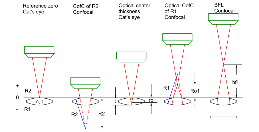
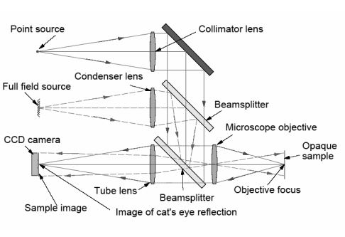
In addition to the laser/fiber combination increasing the resolution, the higher brightness makes the initial alignment of the mirror to the autocollimator easier because the reflected beam is more easily seen under ambient lighting conditions. This angular alignment only concerns two degrees of freedom. To align an autostigmatic microscope that can be thought of as an autocollimator with a microscope objective added on the front, see Figure below, three degrees of translational freedom are involved. This requires even more light to find the location of the reflected spot and get the spot in the small volume of space that the detector can see.

It may seem counterintuitive, but the axial degree of freedom is the most difficult to locate. This is because the focused cone of light spreads out, and its intensity varies as the square of the distance from focus. One must be in the correct axial position to a mm or so to see the focused spot using a 1 mW laser under ambient lighting.

As with the autocollimator, as soon as just a bit of the reflected light enters the microscope objective, the alignment is easy to finish. In fact, with modern digital detectors, the 1 mW source is orders of magnitude too bright to avoid saturated pixels when the reimaged spot is in focus.

In a carryover from past instrument designs, most current autocollimators and centering equipment display an electronic crosshair that simulates what you would see looking into the eyepiece of an older instrument. I prefer to look at the reflected spot image itself because the spot contains information lost with the simulated crosshair. As little as a 10th wave error in the surface being viewed will distort the reflected, nominally perfectly circular spot. Because of this, it is immediately obvious if something is wrong with the object being viewed.

I remember long ago viewing a 300 mm diameter spherical mirror at its center of curvature. The technician behind the mirror adjusting the mount to align the center of curvature to my autostigmatic microscope was surprised when I told him the mirror was too tightly clamped. He said, “That can’t be; it’s only finger tight.” I had him look at the image of three distinct flares at 120° apart. He shrugged his shoulders and said, “Oh,” and went back and loosened the mounting screws.

More recently, much the same thing happened in a government lab using a point source microscope (PSM). The user thought something was wrong with his PSM and had sent me a picture of the image. I suggested he check the mount, and he found that it was the mount, not the PSM, that was at fault. These are examples of situations where if the problem is misunderstood, the error can creep into work farther down the line, where it is even harder to figure out what went wrong. It is much better to find out early, which is easy to do if viewing the real image rather than a simulated crosshair.

[Sidebar] A good reference for looking at images (and that is in print) is Star Testing Astronomical Telescopes by H. R. Suiter, published by Willman-Bell, Inc. (1997). The book has many photographs of star images through focus and of misaligned, poorly mounted and roughly polished surfaces. This gives you a good idea of the kind of images you can see in an autostigmatic microscope that uses a single-mode fiber as a “star.”

There is an additional benefit to directly viewing the reflected image. The same sort of software that aids in aligning astronomical telescopes can be used with a fiber or pinhole-illuminated autostigmatic microscope to give quantitative wavefront information. Here I refer you to
https://www.innovationsforesight.com/product-category/software/skywave/

To recap, the optical principles of modern optical instruments are no different from those used 200-300 years ago. What is different are the sources of illumination, orders of magnitude more intense (the laser or LEDs), and more spatially controlled via optical fibers, computer-generated patterns, and spatial light modulators. On the receiving end, digital cameras are many times more sensitive than the eye. Because of a large range of shutter control, they work well over orders of magnitude of incident intensity. Combining a high-brightness source and the ability to control that intensity at the detector gives modern optical alignment instruments a sensitivity and flexibility that is impossible using the eye as the detector.

In future chapters, we will cover additional flexibility provided by the analysis of structured illumination to provide a third dimension of information from nominally two-dimensional intensity distributions.

[1] Davidson, B. M., “Sources of illumination for the Microscope 1650-1950”, Microscopy, 36, pp. 369-86, (Jan-June 1990)

[2]https://en.wikipedia.org/wiki/Reticle#:~:text=Most%20commonly%20associated%20with%20telescop ic,dates%20to%20the%2017th%20century.

As I said in the first chapter, I hope to make these articles into a book on alignment after significant editing to organize the material coherently. In that spirit, and before I forget, let me discuss some aspects of alignment and precision engineering that belong in a Preface or Introduction to the book rather than here. My motivation is returning from a meeting of the American Society for Precision Engineering, where I took a tutorial on alignment from Vivek Badami of Zygo and Eric Buice from Lawrence Berkeley National Laboratory. You might ask why since I am writing on this subject, but everyone views alignment from a different perspective, and there are aspects of the subject that you might never have thought of but are essential to others. For example, Eric is interested in the alignment of magnets in an accelerator using a wire as the detector of the axis of the magnetic field.

From the alignment tutorial and papers at the meeting, a couple of principles of precision engineering stand out. How well you can make measurements depends on the environment you are working in. At least three significant causes of disturbance exist: thermal effects, vibration, and air turbulence. To give concrete examples, I have attached a paper written several years ago about a large machine tool that illustrates these effects nicely. For each category, I refer to the illustration in the paper. For the details, please see the paper itself.

Thermal effects cause dimensional changes in most materials, and at the µm level and below, people worry about temperature changes of millidegrees. These dimensional changes cause drift and a lack of repeatability. The first example in the paper deals with the lights in the room where the machine was installed. Being conservation-minded folks, we turned the light off in the evening and back on when we got to work in the morning. Unfortunately, this caused an 18 µm change between the tool and workpiece and took most of the workday to stabilize. We just left the lights on all the time, as in Figure 3.

Figure 4 in the paper shows that 0.1° F. change in room temperature will cause a damped reduced temperature of the steel in the machine. The nominal control of the room temperature to 0.02° for several hours was enough to make this a minor contributor to machine errors.

The biggest thermal effect was running the machine spindle. It elongated by 0.5 mm over a 20-hour period. Again, leaving the spindle running except for changing wheels was the only solution, as in Fig 5. In general, thermal effects are categorized as systematic effects; they are relatively long-term effects compared to the time needed to correct for the effect by some feedback mechanism.

In the vibration category, we usually think of seismic vibration coming up through the floor and forget about acoustic vibration. However, even when taking precautions, as shown in Fig. 2, it pays to stay off isolated foundations and avoid touching isolated optical tables during experiments. Leave your laptop off the table and as far away from the experiment as possible. It is a source of vibration and thermal effects.

Acoustic vibrations also have consequences. While I can’t document this, I remember watching a part being diamond-turned at Oak Ridge National Laboratory. They had a claxon to signal for an incoming phone call.  You could see the change in the part’s surface finish from several feet away when the claxon sounded. In another case, having flooring too near the underside of an isolated optical table is a problem. Walking on the floor transfers deflections in the floor to the table because the air between couples the flooring to the table. Here I speak from experience. Opening the gap a couple of inches fixed the problem. The effect of both kinds of vibration combines systematic and statistical noise. Sometimes isolating your experiment from the environment is easy, but just when you think you have it isolated, another source of vibration pops up.

Anyone who has used an interferometer is aware of air turbulence. The irregular change in the shape of the fringes is a sure sign of turbulence. It is also visible in the image using an autostigmatic microscope (ASM). The image’s centroid will dance around, and the flair around the edges of a well-focused spot will change. This type of noise is largely statistical, and the practical method of reducing statistical noise is through averaging. One area of precision engineering that has made large steps here is the astronomical community, which combines wavefront sensing and deformable correction optics to improve the images of stars and galaxies dramatically.

This thought brings me to another impediment to precision, at the µm level, everything is deformable, and to first order, all materials should be considered rubber. Fig. 6 in the paper is a beautiful example.

The ways along which the tool spindle moved were ground steel blocks with a cross-section of 50 by 150 mm. As the spindle moved past the bolts that held the ways together, there was a roughly 10 µm bulge every 150 mm due to over-tightened bolts. Loosening the bolts largely corrected this straightness error. Since the stiffness of plates varies as the thickness cubed, it is easy to see why the least stress will distort thin plates such as lenses and mirrors.

This is probably enough on the difficulty of doing precision work, but it leads to a topic I want to discuss in the next chapter, once you have aligned a system, how do you secure the alignment? The tutorial I attended had a good discussion of this topic, and I will share some of their thoughts in the next installment.

This Chapter is a little out of order but illuminates a topic we have hinted at in previous Chapters, how does the index of refraction affect the lens conjugates we see when doing centration? The immediate interest came from a call I got because some glass apparently got mixed up in a batch of identical lenses. Could I determine which was made of the correct glass? If you are set up to do centering with an optical centering sensor such as an autostigmatic microscope (ASM), the answer is almost always yes. There will be cases where it is impossible for one reason or another, but usually, it is no problem. Note that the same procedure works with an interferometer.

The diagram in Fig. 1 shows the four conjugates you can usually access with an ASM, the green feature being the end of the microscope objective. Notice that these four conjugates allow you to solve for the four first-order lens parameters, the 2 radii, the thickness, and the index.

The leftmost picture shows zeroing the vertical height scale of the ASM on the Cat’s eye reflection from the lens’s upper surface, R2. Once the scale is zeroed, the ASM is lowered in the next picture to pick up the center of curvature of R₂. If R₂ has a long radius, measuring this conjugate may not be possible. The downward motion of the ASM is recorded as a negative distance and matches the normal sign convention for surface radii. If R₂ is concave, the center of curvature is above the surface, and R₂ is positive.

The middle picture is the measurement used to find the index of the glass. The distance, t_o, will always be negative and may be below R₁ if R₂ is sufficiently concave. The next picture shows finding the center of curvature of R₁. Again, R_o1 may be either sign depending on the curvature of R₁, but the distance the ASM moves matches the sign convention of being positive when above the surface.

Finally, if a plane mirror is placed behind the lens, we can find the back focal length (BFL), which may be either positive or negative depending on the 2 radii. In these last 2 cases, the distances may be out of reach with negative lenses. The good news is that if the lens is turned over, most previously inaccessible conjugates are now accessible.

The pictures are ordered toward a more complicated formula for finding the conjugate. Left most we just set our scale to zero. The radius of R₂ is confocal, so no calculation is needed; the measurement is independent of any other lens parameter. Obviously, the objective must have a long enough working distance to reach the center of curvature. When this is not the case, turning the lens over and measuring from the other side may solve this problem.

The optical thickness is

where t_p is the physical thickness of the lens, and 3 of the 4 lens parameters are used. This can be turned around to give the index as

Notice this formula gives the same index n either way the lens is facing because t_o and R₂ both change when the lens is inverted. This gives 2 measures of the index from one lens. Also recognize that in the limit of large R₂, that is, a plane window, the formula reduces to n = t_p/t_o just as we expect.

To find the optical center of curvature of R₁ it requires all 4 lens parameters.

Notice that odd things happen if R₁, the surface farthest from the ASM, is plane. This formula says that the optical radius of R₁,in the limit as R₁ goes to infinity, is

This is the same as the back focal length, BFL, and the EFL for a plano-convex or concave lens when the plano side is farthest from the ASM. In practice, there is one focused spot behind the lens where we cannot tell the difference between the three. This is less confusing when we remember we are not measuring the physical radius of curvature but rather where the center of curvature of R₁ appears relative to the vertex of R₂. R₁ must be substantially non-plane before the three spots are separated enough axially to distinguish between the EFL, BFL and optical radius of R₁.

Finally, the BFL also uses all four lens parameters.

The reason for calculating R_o1 and BFL is that once you have found the index, you can substitute the index in these formulas and see if you get these conjugates when you measure the lens as a double check on the index, and to see if you have made any mistakes (particularly, sign errors) along the way.

While I was prompted to write this Chapter because of a concern with the index of refraction, you can see the direct association with alignment. For every lens added to an assembly, you can pick up these four conjugates unless they happen to be too large to reach with the hardware available in either direction relative to the zero of the surface nearest the alignment sensor. Obviously, the more lenses in an assembly, the more surfaces and centers of curvature are going to show up as you scan through the lens axially. This is why it is good practice to have a list of conjugates of a correctly assembled lens before inspecting it. If you do not have such a list, it is difficult to know which spot is reflected from what conjugate.

[Sidebar – There is a second method of finding the axial location of the center of curvature of a surface that is particularly useful when using a lens design program. Rays reflecting from the surface in question are normal to the surface to focus at a point. According to Snell’s Law of Refraction nsin(Ø) = n’sin (Ø’) where Ø and Ø are measured relative to the normal of the surface. The Law means that Ø’ is zero for rays normal to the surface. If n = 0, then Ø’ is 0.

This observation is helpful because to find the location of a surface’s reflected center of curvature; the designer must enter all the surfaces between the sensor and the reflecting surface twice. The n = 0 method is single pass approach for a source at any distance from the surface on to the sensor as long as n = 0 just prior to the surface. Simulating the suitability of any reflecting test is easy. After finding a suitable solution, the system is modeled in double pass to verify a correct design. Try the method. You will be amazed how much easier it is to do this than set up a double pass test.

I cannot take credit for this idea. I believe I heard it from Jim Burge, and I suspect he heard it from Roland Shack.]