This Chapter is a little out of order but illuminates a topic we have hinted at in previous Chapters, how does the index of refraction affect the lens conjugates we see when doing centration? The immediate interest came from a call I got because some glass apparently got mixed up in a batch of identical lenses. Could I determine which was made of the correct glass? If you are set up to do centering with an optical centering sensor such as an autostigmatic microscope (ASM), the answer is almost always yes. There will be cases where it is impossible for one reason or another, but usually, it is no problem. Note that the same procedure works with an interferometer.
The diagram in Fig. 1 shows the four conjugates you can usually access with an ASM, the green feature being the end of the microscope objective. Notice that these four conjugates allow you to solve for the four first-order lens parameters, the 2 radii, the thickness, and the index.
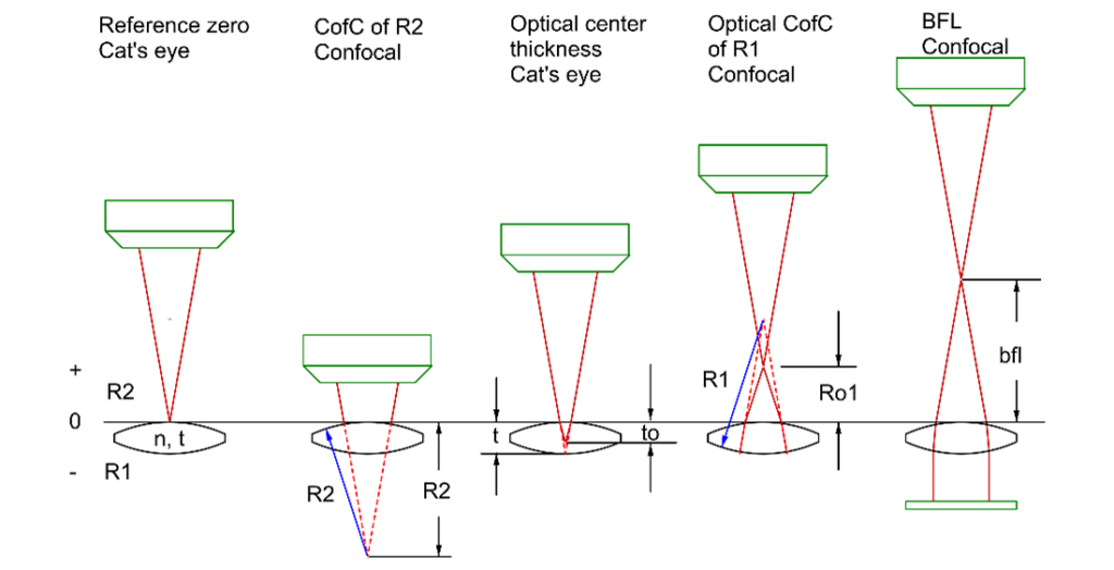
The leftmost picture shows zeroing the vertical height scale of the ASM on the Cat’s eye reflection from the lens’s upper surface, R2. Once the scale is zeroed, the ASM is lowered in the next picture to pick up the center of curvature of R2. If R2 has a long radius, measuring this conjugate may not be possible. The downward motion of the ASM is recorded as a negative distance and matches the normal sign convention for surface radii. If R2 is concave, the center of curvature is above the surface, and R2 is positive.
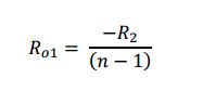
The middle picture is the measurement used to find the index of the glass. The distance, to, will always be negative and may be below R1 if R2 is sufficiently concave. The next picture shows finding the center of curvature of R1. Again, Ro1 may be either sign depending on the curvature of R1, but the distance the ASM moves matches the sign convention of being positive when above the surface.
Finally, if a plane mirror is placed behind the lens, we can find the back focal length (BFL), which may be either positive or negative depending on the 2 radii. In these last 2 cases, the distances may be out of reach with negative lenses. The good news is that if the lens is turned over, most previously inaccessible conjugates are now accessible.
The pictures are ordered toward a more complicated formula for finding the conjugate. Left most we just set our scale to zero. The radius of R2 is confocal, so no calculation is needed; the measurement is independent of any other lens parameter. Obviously, the objective must have a long enough working distance to reach the center of curvature. When this is not the case, turning the lens over and measuring from the other side may solve this problem.
The optical thickness is
where tp is the physical thickness of the lens, and 3 of the 4 lens parameters are used. This can be turned around to give the index as
Notice this formula gives the same index n either way the lens is facing because to and R2 both change when the lens is inverted. This gives 2 measures of the index from one lens. Also recognize that in the limit of large R2, that is, a plane window, the formula reduces to n = tp/to just as we expect.
To find the optical center of curvature of R1 it requires all 4 lens parameters.
Notice that odd things happen if R1, the surface farthest from the ASM, is plane. This formula says that the optical radius of R1,in the limit as R1 goes to infinity, is
This is the same as the back focal length, BFL, and the EFL for a plano-convex or concave lens when the plano side is farthest from the ASM. In practice, there is one focused spot behind the lens where we cannot tell the difference between the three. This is less confusing when we remember we are not measuring the physical radius of curvature but rather where the center of curvature of R1 appears relative to the vertex of R2. R1 must be substantially non-plane before the three spots are separated enough axially to distinguish between the EFL, BFL and optical radius of R1.
Finally, the BFL also uses all four lens parameters.
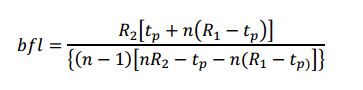
The reason for calculating Ro1 and BFL is that once you have found the index, you can substitute the index in these formulas and see if you get these conjugates when you measure the lens as a double check on the index, and to see if you have made any mistakes (particularly, sign errors) along the way.
While I was prompted to write this Chapter because of a concern with the index of refraction, you can see the direct association with alignment. For every lens added to an assembly, you can pick up these four conjugates unless they happen to be too large to reach with the hardware available in either direction relative to the zero of the surface nearest the alignment sensor. Obviously, the more lenses in an assembly, the more surfaces and centers of curvature are going to show up as you scan through the lens axially. This is why it is good practice to have a list of conjugates of a correctly assembled lens before inspecting it. If you do not have such a list, it is difficult to know which spot is reflected from what conjugate.
[Sidebar – There is a second method of finding the axial location of the center of curvature of a surface that is particularly useful when using a lens design program. Rays reflecting from the surface in question are normal to the surface to focus at a point. According to Snell’s Law of Refraction nsin(Ø) = n’sin (Ø’) where Ø and Ø are measured relative to the normal of the surface. The Law means that Ø’ is zero for rays normal to the surface. If n = 0, then Ø’ is 0.
This observation is helpful because to find the location of a surface’s reflected center of curvature; the designer must enter all the surfaces between the sensor and the reflecting surface twice. The n = 0 method is single pass approach for a source at any distance from the surface on to the sensor as long as n = 0 just prior to the surface. Simulating the suitability of any reflecting test is easy. After finding a suitable solution, the system is modeled in double pass to verify a correct design. Try the method. You will be amazed how much easier it is to do this than set up a double pass test.
I cannot take credit for this idea. I believe I heard it from Jim Burge, and I suspect he heard it from Roland Shack.]