EXPERIMENTAL SETUP:
A Point Source Microscope (PSM) was mounted on a motorized vertical stage above a 25 mm diameter, 200 mm efl lens sitting above a plane mirror. A square black paper mask with an 8 mm diameter hole was placed over the lens as shown in the figure below to give an f/25 aperture.
BACKGROUND:
I was asked, “How well can the PSM find best focus of slow optical system?” In particular, could best focus be determined to ± 10 μm on an f/25 system? Conventional wisdom would say this is not possible as the depth of focus is on the order of λ(f/#)^2, something like 400 μm in this case. On the other hand, conventional theory claimed sub-micron microscopy in the visible was not possible until the invention of confocal microscopy. The answer for me was to try an experiment.
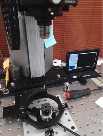
(The black ring mirror mount surrounding the lens and mask where used in another experiment.) The PSM had a 4x microscope objective attached.
After centering the lens to view the back focus in the center of the PSM video monitor, the PSM was scanned vertically over a range of about 1 mm while collecting and storing data about the reflected image every 4 μm for a total of about 264 points per scan.
The centroiding algorithm in the PSM looks at pixels more intense than a user set threshold. The threshold was set to about 125 out of an 8 bit range of 256. When the PSM is used for alignment, the centroiding algorithm calculates the center of gravity of those pixels above the threshold. The software also records the number of pixels above the threshold at each point in the scan. The shutter speed or exposure was user set so there were about 35 pixels above the threshold near best focus.
The limits of the 1 mm scan were then set to give a roughly symmetrical distribution of pixels around best focus so that a typical scan gave a curve in Excel like that below.
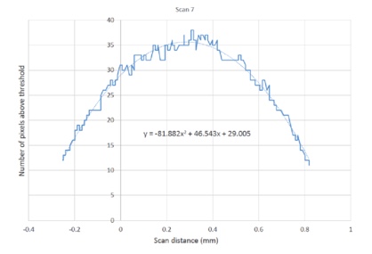
Using the curve fitting options in Excel, a quadratic curve fits well as expected. If the criterion for best focus is taken as the distance where there are the greatest number of pixels above the threshold, then taking the derivative of the equation and setting it to zero gives x = 0.2842 mm. The data are a bit noisy but the results look promising.
Much to my pleasant surprise, the other 9 repeated scans looked very much the same. The results are summarized in Table 1.
| 3 | y = -84.213×2 + 48.431x + 29.412 | 0.2876 |
| 4 | y = -82.682×2 + 46.997x + 29.391 | 0.2842 |
| 5 | y = -82.427×2 + 46.602x + 29.297 | 0.2827 |
| 6 | y = -84.332×2 + 47.958x + 29.28 | 0.2843 |
| 7 | y = -81.882×2 + 46.543x + 29.005 | 0.2842 |
| 8 | y = -82.67×2 + 46.447x + 29.301 | 0.2809 |
| 9 | y = -82.649×2 + 46.619x + 29.445 | 0.2820 |
| 10 | y = -84.167×2 + 47.557x + 29.56 | 0.2825 |
| 11 | y = -81.648×2 + 46.481x + 29.519 | 0.2846 |
| 12 | y = -81.92×2 + 46.969x + 29.705 | 0.2867 |
Table 1 The scan number, equation of fit to the number of pixels above threshold vs focus position and the position of best focus in mm
Ten scans through focus were taken under identical conditions, that is, over the same distance with the same threshold and exposure. The data from the scans were fit to second order polynomials as in the Scan 7 picture, and the coefficients of the fit are displayed in Table 1. Solving for the best focus position, defined as the position where there are the most pixels above the threshold gave an average best focus position of 0.2840 ±0.0020 mm.
These encouraging results must be viewed with two caveats; the test for finding best focus was a double pass test off a plane return mirror so single pass results will be less precise by a factor of two. The other caveat is the definition of what constitutes best focus, this may not be best focus in terms of best resolution for a particular spatial wavelength. However, it is a useful definition if it is desired to see if multiple examples of the same optical system behave similarly to a measurement of best focus.
The conclusion of this simple experiment is that the PSM can find best focus for an f/25 lens in double pass transmission with a standard deviation of 2.0 μm when axially stepped multiple times through the region of focus. Each scan took about 5 seconds, and the fitting and analysis of the data from multiple scans are easily automated