Author: csadmin
Chapter 16 – Footnote for Chapters 14 and 15
This brief chapter serves as a vital addendum to the last two chapters. While I’ve already described the alignment process, I realized I hadn’t emphasized how remarkably simple it is—and what makes it so effortless. Over the years, countless methods have been used to align optics successfully, long before Bessel beams entered the picture. What makes this approach truly stand out isn’t just its precision, though it certainly delivers that—it’s the unparalleled ease and speed with which it is done.
Let me begin with a brief review. We create and project a Bessel beam as a reference axis. We view the beam using a Point Source Microscope (PSM), and it is aligned to the PSM reference crosshair. We assume that the crosshair has been pre-aligned using a Cat’s eye reflection so that it is conjugate with the point source in the PSM.
The alignment task is to insert an optical system into the Bessel beam such that the beam is undisturbed from its initial condition, that is, the beam propagates through the system with no change in position or angle. This means the optical axis of the optical system must be coaxial with the Bessel beam reference axis. Because we must align an axis, we must be able to view two points along the axis that are separated axially; the farther the separation, the more sensitive we are to the misalignment of the axis.
Traditionally, this was accomplished using an alignment telescope, which was first focused at one point, and the system moved to bring the point onto the crosshair. Then, it was focused on the second point, where that position was aligned. Because, in practice, you seldom rotate or translate about optimum locations due to hardware constraints, the alignment proceeds gradually as one step slightly misaligns the previous step. And because of the refocusing between steps, you tend to forget which direction you moved in the previous step once removed; you often find yourself repeating yourself, sometimes going backward. The process is tedious, frustrating, unproductive, and prone to error.
When using the Bessel beam and PSM combination, the Bessel beam is visible on the PSM camera anywhere along the beam. In addition, the PSM generates a point source at the focus of the objective. As the PSM is moved along the Bessel beam, the focus of the objective can be positioned at the center of curvature of an element in the optical system. When it is focused there, a reflection from the center of curvature is also visible on the camera. This gives two spots associated with the system undergoing alignment to work with simultaneously. These concepts are illustrated in the schematic figure below.
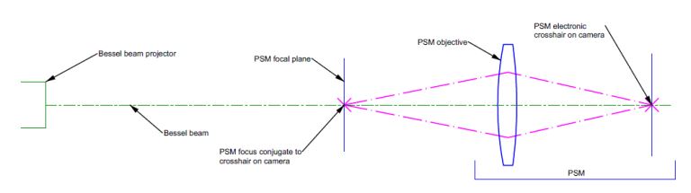
This figure schematically represents the PSM aligned to the reference Bessel beam prior to the insertion of the optical system to be aligned to the beam. The electronic crosshair is aligned to the stigmatic focus of the light exiting the PSM objective to < 1 um precision by viewing a Cat’s eye reflection off a specular surface. The PSM is then centered to the Bessel beam to 1 um precision at an axial location that is conjugate to an accessible center of curvature in the system to be aligned to the Bessel beam. Once this initial alignment of the Bessel beam/PSM pair is complete, the system to be aligned is inserted between the projector and the PSM, as in the next diagram.
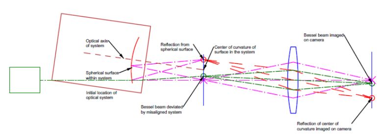
Inserting the system deviates the Bessel beam, so it is no longer centered on the PSM crosshair. Additionally, the light from the PSM’s stigmatic focus is reflected in the system’s spherical surface. It refocuses on the PSM focal plane displaced from the stigmatic focus because the system is tilted relative to the initial Bessel beam axis. These two spots are reimaged on the camera displaced from the electronic crosshair. It is now a matter of translating the system to bring the Bessel beam to the crosshair and then tilting the system to bring the reflection from the spherical surface to the crosshair. This tilting will slightly move the Bessel beam from the crosshair, so the alignment process must be iterated. However, we have shown that the process converges to the PSM’s resolution limit in 3 to 4 iterations. In the end, we have the situation pictured below.
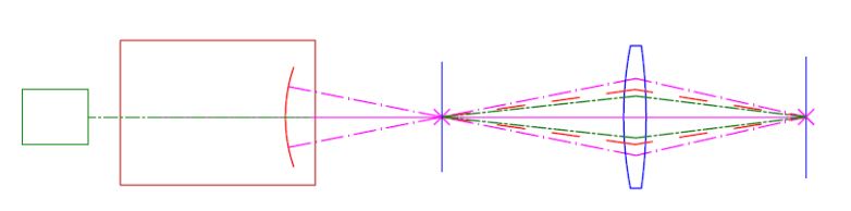
The center of curvature and the Bessel beam lie on the PSM crosshair and are coincident at the objective focus with the exiting stigmatic focus to < 1 um on the PSM with a 10x objective.
Seeing both spots simultaneously makes it significantly easier and faster to center them to the reference crosshair of the PSM. Because the system’s geometry is the same as using an alignment telescope, the movement of the spots with adjustments to the system may still be confusing. The spots may move in opposite directions as the optical system is adjusted, or one spot may move much faster than the other. However, it is easy to make small adjustments and continuously track both spots without touching the PSM.
This allows you to focus exclusively on aligning the system in translation and tilt with direct, real-time feedback, which is the most important advantage of the PSM/Bessel beam method. The continuous, direct feedback from both spot positions makes the method fast and completely deterministic while maintaining or improving the precision of using an alignment telescope. If you go to this 1 minute YouTube video https://youtu.be/UKSTej0Xt5k you can see just how fast the process is. The clip is taken out of context so there is no audio, but you can see the Bessel beam initial and then the spot from the center of curvature. The brief pause was to correct the relative intensities of the spots and change the screen so you can see the x,y coordinates of the centroid of the spots on the screen in µm.
Chapter 15: Tabletop Alignment Part 2
In Chapter 14, we showed how to determine the axis of a laser beam to which we want to align optical elements and then how to align a Bessel beam to the laser beam axis. This Chapter shows the steps to align optical elements to the reference Bessel beam. With tabletop alignment, you have all five degrees of freedom necessary to achieve complete alignment in translation and tilt. The only constraints to eliminating all alignment errors are the resolution of your alignment metrology instrument and the mechanical resolution and stability of your optical mounts.
Although you can achieve full alignment on a tabletop, the process is more complex than placing lenses in a cell because the lens cell explicitly defines some of the degrees of freedom that constrain the lenses. Often, these constraints make it impossible to achieve full alignment in an assembly of lenses. On the tabletop, although you have all the necessary degrees of freedom, you must have a procedure and methods of providing datums for the five degrees of freedom required to get full alignment. This Chapter explains the procedure and methods.
Figure 1 schematically shows the steps required before aligning the first element in a chain of elements. Following this overview, we will break the procedure into individual steps and explain each. To keep this simple, the example assumes a 2-element, 3:1 beam expander starting with the positive element. Once we have covered the initial preparations, we show the element’s alignment to the reference axis.
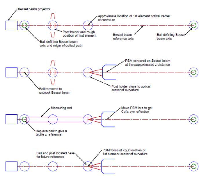
Fig. 1 Alignment steps before inserting the 1st element, shown in its intended position in dashed lines into the Bessel beam
In Chapter 14, we had the Bessel beam projector aligned to the laser beam axis. From our plan to introduce a 3:1 beam expander, we know that the optical center of curvature of the lens’s first surface must lie on the axis of the Bessel beam at a specific z distance along the beam. Fig. 2 shows the preparation for this step, where we roughly locate a post holder for the 1st element and another for the ball at the optical center of curvature using the tapped holes in the tabletop and a ruler for guidance.
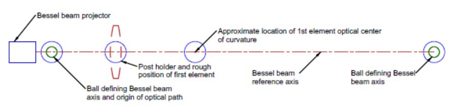
Fig. 2 Post holders roughly centered on the Bessel beam axis the approximate z distances required
Once the post holders are located and secured, we align a PSM to the Bessel beam in x, y, as in Fig. 3, with its focus above the center of a post in the holder for the ball.
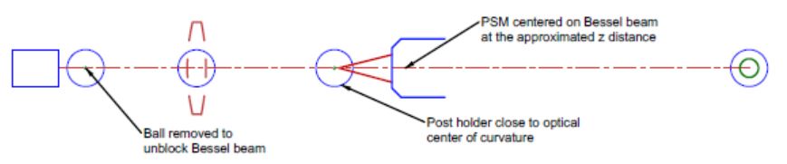
Fig. 3 The PSM is centered on the Bessel beam after removing the ball blocking the beam
With the PSM centered on the Bessel beam to < 1 µm in x and y, the reference ball near the projector is replaced on its post to serve as a tactile reference to establish the z distance to the optical center of curvature as in Fig. 4.
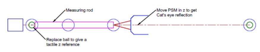
Fig. 4 Establishing the correct z distance to the optical center of curvature
The measuring rod in Fig. 4 could be a custom rod with square ends just for this spacing, an inside micrometer, or calipers. The measuring device or rod should be held in a stable mount for the most precise spacing. The lens post holder could be used temporarily for this purpose. When the rod touches the reference ball, the PSM is moved in z until the Cat’s eye reflection from the rod end is in good focus. Now, the PSM focus defines a point in space accurate to 1-2 µm in three degrees of freedom that will be the location of the optical center of curvature of the lens’ 1st surface when the lens is inserted.
Then, remove the ball and measuring rod to ensure the PSM is still well centered in x and y. Since this will be a reference for the beam expander, adjusting a post and ball here for the future is good practice, as in Fig. 5. There is no need for an adjustable mount. The post holder may be tapped into position using the two degrees of freedom provided by the tabletop, and adjusting the height by squeezing the post with thumb and finger against the top of the post holder, as in pulling a tooth, after slightly loosening the locking screw. With a little patience, this can be done with a precision of a micrometer or two.
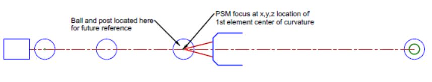
Fig. 5 Ball located at the optical center of curvature of the first surface of the positive element
Now, the PSM focus is located in three degrees of freedom, ready for the positive element to be inserted. Notice that the PSM defines five degrees of freedom for the lens, two degrees for the x, y location of the Bessel beam transmitted through the lens, and, separately, in three degrees that define the optical center of curvature.
Fig. 6 shows the situation when the lens is inserted and then the first iteration of alignment. We show a case where the lens is inserted 2 mm decentered and 2° tilted. You can probably do better than this by eye, but then it would be difficult to illustrate the alignment in the Figure.
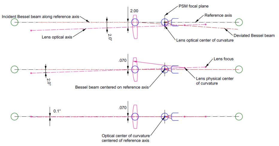
Fig. 6 The first lens is inserted in the Bessel beam and the first iteration of alignment
The inserted lens’s tilt and decenter cause the Bessel beam to deviate, so the PSM sees the beam below the reference axis. The optical center of curvature lies farther from the reference axis. The first alignment step is shown in the middle view when the lens was moved upward 1.93 mm so that the Bessel beam is centered to the PSM to < 1 µm. This first step of centering the lens leaves the vertex of the first surface 0.07 mm below the reference axis and moves the optical center of curvature above it by 0.405 mm because the lens’s tilt is unchanged.
In the lower diagram, we tilt the lens 1.9° to bring the optical center of curvature so it is centered to the PSM. It looks in the figure like we are about done. However, because the vertex of the lens is 0.07 mm below the reference axis, there is still about 0.1° of tilt, which makes the Bessel beam decentered by 11 µm below the axis. We can do better by repeating this same sequence of alignment operations until the Bessel beam and optical center of curvature are < 1 µm from centered to the PSM.
Since the process converges rapidly, about a factor of 3 to 4 per iteration cycle, and the PSM is not touched during the alignment process, the lens alignment is faster than preparing to do the alignment. Just three to four cycles of alignment center the lens to < 1 µm and < 1 second of arc. This means the Bessel beam is deviated by no more than this so it is used as the reference axis for inserting the negative lens in the beam expander.
Several details need to be mentioned. We have assumed the lens mount rotates the lens about its first surface, where most 5-degree-of-freedom mounts pivot. The convergence ratio depends on where this pivot lies and is fastest when the pivot is in the plane of the lens’s second surface. During the centering and tilting, the adjustment screws will shift the z distance of the lens, leading to a defocus. Your adjustable lens mount should have an adjustment screw at the pivot point, making it fully a five DOF mount so the z spacing can be controlled by adjusting all three screws and correcting the defocus.
I finish this Chapter on 5 degree of freedom lens alignment by referring you to a video of this type of alignment, but in a different context. The video shows the meniscus half of a cemented doublet being aligned before adding the positive element for cementing. During the alignment, the seat for the meniscus is centered by tapping to align the lens in translation. At the same time, it is rotated or tilted by sliding it on the seat, again by gentle tapping, to bring the center of curvature centered to the PSM.
In the video, you will see that tapping sometimes overshoots, but with a little patience, you can center the seat to 1 µm and get the tilt to about 1 arc second, depending on the radius of the surface in the seat. Further, there is instant eye/hand feedback, so it is immediately obvious where the next tap should go. It is also evident that the process could be automated should the quantity of lenses warrant the expense.
https://vimeo.com/818873649/d7b8444277 Fast-forward to 14:30 to see the lens first inserted into the Bessel beam, then go to 16:00 to see additional centering. Open the video to full screen so you can see the numbers showing the centration in µm. Once you watch the video part, you may want to read the introductory material that explains the full process and why there are constraints when centering lenses in a cell.
Chapter 14: Tabletop Alignment Part 1
At last, I am back to writing more about optical alignment. The hiatus was due to my realization that most readers are not interested in assembling lenses in a tube. Rather, they want to align free-standing optics on tabletops or benches in labs researching topics like laser light interactions with matter, free-space communication, and quantum computing. The picture below shows what I mean. It took time to rearrange my thoughts.
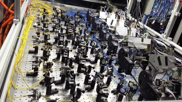
(Picture credit: Figure 2 from Anastasi, A., Basti, A., Bedeschi, F., Boiano, A., Bottalico, E., Cantatore, G., Cauz, D., Chapelain, A.T., Corradi, G., Dabagov, S. and Di Falco, S., “The laser-based gain monitoring system of the calorimeters in the Muon g−2 Experiment at Fermilab”, Journal of Instrumentation, 14(11), p. P11025, (2019))
To achieve maximum performance from such tabletop laser systems, that is, to get the maximum irradiance (W/m2) on the target, the optics must be aligned to tolerances that approach or surpass those for lenses in a cell. However, finding references to the precision alignment of such tabletop systems is difficult. The break in writing was to investigate this type of alignment where it is impossible to use an axis of rotation as a reference axis.
The investigation led to several constructive conclusions: with tabletop alignment, you always have the 5 degrees of freedom to align the optical axis of a component to your reference axis, which is often limited to only 2 or 3 degrees of freedom in the case of lenses in a cell. This means you can achieve perfect alignment to the resolution limits of your ability to adjust the optics and your alignment detection system. Further, the method of alignment using a Bessel beam has already been shown effective and reported [1], but not in the context of tabletop alignment. The method is perfectly suited to tabletop alignment. Finally, Glen D. Gillen’s well-written tutorial introduction to tabletop alignment is freely available online [2]. I encourage reading this as it has many practical tips to consider before starting benchtop alignment.
To start the alignment of getting a laser beam from a source to a target, we must find the laser beam’s axis and then align our reference Bessel beam axis to it. Next, we must generate the Bessel beam to align the first lens in the path using an autostigmatic microscope. This chapter will cover these two topics and leave the lens alignment for Chapter 15.
Aligning a Bessel beam to a laser beam
For a low-power laser, use a quadrant detector to locate the center of the beam at two locations along the beam. Once the quadrant detector is centered on the beam, bring an autostigmatic microscope up to it and center the PSM on the intersection of the quadrants. Remove the quad cell and replace it with a ball on a post so the center of the ball is at the PSM focus. The ball marks one point along the beam. Repeat this with the quad cell at a second location along the beam and use the PSM to position a second ball at the center of the quad cell. Now, the path of the laser beam is known in position and angle.
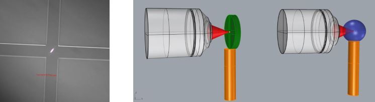
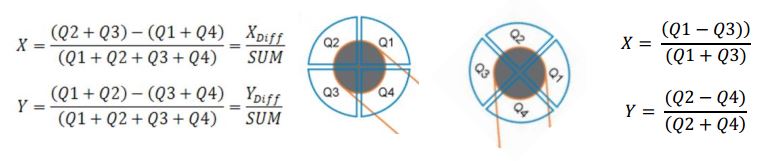
Left, center of quad cell as seen by the PSM. The gap between quadrants is 100 µm, and the white spot in the middle of the gap is the Cat’s eye reflection from the cell surface as seen through the imperfect window on the quad cell. Right, the PSM objective focused on the quad cell intersection. Then, the quad cell is removed, and a ball is centered on the objective focus to transfer the location of the cross.
Sidebar: Use quad cells wisely, at 45° to the tabletop. Then, the beam location is the difference of the opposing quadrants. This is easier than placing the quad cell square with the table where the voltages from pairs of quadrants must be added before they are differenced, as seen in the figure.
For a high-power laser, burn a spot in a card placed in the beam and use the PSM to focus on the center of the burn spot. Use the PSM to position a ball as in the quad cell case. As with the quad cell, a second spot along the beam must be found to establish the beam axis. Now, the two balls define the axis of the laser beam.
Sidebar: Note that a quad cell is useless for centering a Bessel beam. Because the energy in each ring is the same as the core, or any other ring, the average intensity of the Bessel beam is essentially constant, so the quad cell sees little change as the Bessel beam moves across it.
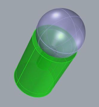
Creating and aligning the Bessel beam
Although Bessel beams were discussed in Chapter 9, I did not specifically say how I was producing them. I use chrome on glass zone plates (equally spaced, concentric circles) made by photolithography techniques [3] with 20 µm line pair spacing to give a diffraction angle of about 1.8° when illuminated with 635 nm light. The zone plate is illuminated with a single-mode optical fiber located about 200 mm behind the grating. This set of conditions produces a Bessel beam that starts within a few µm of the grating and extends for meters with a 25 mm diameter grating.
Catalog item Axicons also create Bessel beams, which single-mode fibers can illuminate to produce long Bessel beams. I prefer fiber rather than collimated illumination because no collimating lens is needed, making the setup simpler and allowing the Bessel beam to propagate farther. Also, I like the grating zone plate because it is easier to align the beam normal to the grating, and the grating also serves as a plane mirror in its zero-order mode. Either way, an Axicon or zone plate grating defines 5 degrees of freedom with one optical element.
We return to the two balls defining the laser beam to align the Bessel beam with the laser beam axis. Assuming the balls are mounted kinematically (see Sidebar) to be removed and replaced repeatably, the PSM is focused on the center of the ball farthest from the Axicon or grating. Then, the ball is removed, and the Bessel beam projector is rotated until the Bessel beam is centered on the PSM. The ball nearest the projector is placed on its mount, and the PSM is centered on the ball, and the ball is removed. Then, the projector is translated to bring the BB onto the center of the PSM. This cycle is repeated until the beam is centered on both balls. The process is a bit tedious. However, since it is possible to center the beam to <1 µm and if the balls are 200 mm or more apart, the BB will be coaxial with the laser beam to .002/200 = 1e-5 = 2 arc seconds.
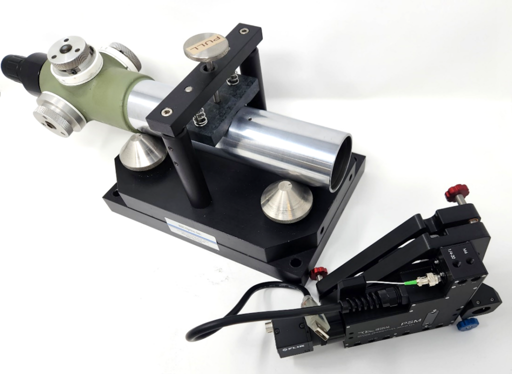
Sidebar: An easy way to mount balls that define mechanical datums is to set them on the ends of lens posts used for mounting stand-alone optics. The lens posts typically have a countersunk conical bore, as in the picture, that serves as a seat for a ball of roughly the same diameter as the post. With good quality balls the center of the ball will repeat its location to < 1 µm each time it is removed and replaced. By good quality ball, I mean Grade 5, round to 125 nm. If worse quality balls are used the reflected image may seem displaced by more than the repeatability of the kinematic mounting. There are precision, magnetic holders designed for use with the SMR retroreflectors employed with laser trackers for non-vertical locations. These mounts, or nests, are expensive compared to lens posts.
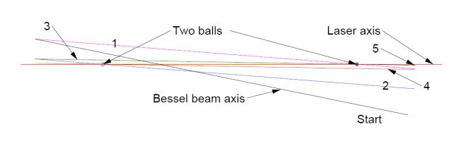
The line figure shows the horizontal laser axis (red line) and the Bessel beam axis at the start of the alignment (black line). The numbers show how the alignment proceeds by rotating the axis to the ball farthest from the point of rotation until the axis is aligned with the ball, step 1, and then translated to align with the near ball, step 2, etc. The convergence occurs rapidly, even though the PSM has to be moved between iterations.
Once the reference Bessel beam is aligned with the laser axis, we are ready to align lenses to the beam, the subject of Chapter 15.
References
[1] R. E. Parks, Precision cementing of doublets without using a rotary table, Proc. SPIE, 11487OU (2020)
[2] Gillen, Glen D. “Laser Laboratory Beam Alignment Skills: Course Package.” arXiv preprint
arXiv:2404.16225 (2024).
[3] Bessel beam zone plates are made by Arizona Optical Metrology, LLC, https://aom.us/
Chapter 13: New Optical Alignment Tools
In Chapter 12, I commented again on classical optical instruments since there was interest in an earlier discussion. This got me thinking about what had changed in optical technology since the period ending about 1950 when there was a rather canonical set of classical optical metrology tools. There has been a huge technological change since then, yet little has been written about coherently integrating the changed pieces of technology. That is what I am going to try to do in this Chapter.
Virtually all optical systems have three major components: a light source, some optics that modify the light from the source, and a detector. I will address the changes in these three areas separately to give some order to the discussion and then summarize the consequences of the changes in designing new optical metrology instruments.
Light sources
In the years before the laser, that is, before 1960, man-made sources were either incandescent or some sort of electrical arc. Incandescent sources were physically large and not very bright but fairly stable in terms of position and intensity. Arc sources were brighter or could concentrate their brightness into a smaller size but were much harder to control in terms of the location of the brightness and its intensity level. Even when the HeNe laser came along and solved the brute intensity issue, workers went to great lengths to create point sources by using a microscope objective and a pinhole to “clean up” the source.
Today, I can create a bright, to-the-point-of-eye safety concerns, essentially perfect spherical wavefront with a single-mode optical fiber patch cord and a battery-operated 30 mW LED source used for testing optical fibers for continuity that sells for $20. (See, for example https://www.amazon.com/AKLTM-Visual-Fault-Locator-Tester) The only practical downside to this source is that it is too bright for some applications, and the intensity is not adjustable. There are commercially available laser diode sources that are perfect for illuminating a single-mode fiber, are fully adjustable from pW to mW, and are available in various wavelengths from NUV to NIR. These low-power, adjustable sources typically cost 50-100x the battery-operated ones, but you have control and stability.
Optical elements
Between the source and detector are optics that modify the light before it reaches the detector. Various optical elements could go here, but I will stick to lenses and mirrors. About the time of the invention of the laser, you could begin to buy lenses out of a catalog, with Edmund Optics leading the way. This made it much easier for someone to try out a particular combination of lenses on an optical bench to prototype a new system without waiting for custom (and expensive) optics to experiment with.
Another development starting about the same time was computer-aided lens design. This meant there was more variety in optical systems that could be assembled without much expense and delay because designing new optical systems was easier. This development led to a commercial market for impressive photographic camera lenses. At the same time, governments realized it was much easier to spy on everyone with sophisticated telescopes in planes and satellites.
This, in turn, led to testing optics interferometrically to make better-quality optics than previously. Once testing was easy, there was a push toward deterministic polishing methods, such as the MRF technique developed by QED Technologies. This meant that the lenses listed in catalogs were sufficiently high quality that diffraction-limited systems could be laid out on a tabletop optical bench. The only obstacle to diffraction-limited performance was the precision of the optics’ alignment.
Detectors
Before about 1970, most images were captured on photographic film, a reliable and inexpensive method of capturing and storing massive amounts of data. However, if your camera loaded with film was in space and you wanted to see the pictures, there was a problem. The other demand came from photographers with expensive lenses who wanted to see the results of their pictures sooner rather than later. This led to the development of electronic cameras, but because they used the newest technology, they were pricey. If you had a spy satellite or a large terrestrial telescope, you could afford an electronic camera, but they were not affordable for the general public before about 2000.
For scientific use, electronic cameras are incredibly useful. An easily affordable megapixel camera with a shutter speed range of microseconds to seconds and additional gain was readily available by 2005. Such a camera coupled with microscope optics was capable of diffraction-limited imaging with a 10 x objective over a 1 mm square field of view with instant image availability for further processing. One could argue that photographic film has a higher data storage density than an electronic camera. However, in conjunction with its associated computer, the electronic camera is so much more flexible as a data interface that it is the obvious choice for data capture.
The whole is greater than the sum of the parts
When you consider an autocollimating or autostigmatic optical instrument that incorporates a light source, optics to project and receive light from the source, and a camera to capture and store the image, you now have much more to work with than they did in the day of the classic instruments. Between the adjustability of the light source and the camera you have a useful range of intensity variation of something on the order of 1010. The data cube in one megapixel, 16-bit image is in the same order.
During initial alignment to get reflected light into the instrument, you can turn the laser to its maximum 1 mW level for a Class 1 laser device and see the light under many ambient lab lighting conditions, so you don’t have to darken the lab to find the light. Once the light is back in your instrument, you don’t have to work your head into an odd angle to view in an eyepiece; you can comfortably observe the image on a monitor. Finding a zero setting or finding coincidence is no longer subjective; you get a repeatable, objective number on a monitor. You don’t have to write down your measurement result; you tap a key to store the result or the whole image on a computer that controls the instrument.
Implication of technological changes on the mechanical design of classic optical instruments.
If you knew nothing about the design considerations of classical optical metrology instruments, think of autocollimators as an example, but had today’s technological resources, would you design an autocollimator to look like a classic example? I argue, no. Would the new instrument have a large aperture? No. You get plenty of light back into a small aperture with a laser source.
Would you use a round, precision-ground barrel as a mechanical datum to aid in setting the crosshair to the center of the aperture? No, you can set zero by pointing the instrument at a small retroreflector. Would you use an incandescent light source that draws 10 or more Watts or a laser diode that draws 10 mW? Would you use the new technology for light sources and cameras but then attach it to a custom controller for readout? No, you would attach your device to a generic computer via a USB cable and put the custom controller and readout into the software on the computer.
I conclude that with the new technology, classical optical instruments can retain their same function and accuracy without requiring the older instruments’ mass, size, external features, and electrical demands. No, the new instruments will not look the same as the old or be massive, yet they will perform the same function as well or better than the old. The hurdle is to set aside the picture of a classic autocollimator and ask where is the modern functional equivalent. Optical metrology instruments using the new technology are now catalog or online store items.
The old and the new with greater functionality using today’s technology