New Product Launch
Optical Perspectives Group proudly introduces PSM Align
Revolutionary Python-Based Software for Point Source Microscope
Now Standard on All PSM Units

Author: csadmin

Ritchey-Common Test & Similar Methods Using AI Image Space Phase Retrieval

In this document, we will describe a general approach/method to measure optical surfaces in reflection and/or transmission when the incoming beam is not a simple plane wave. Among such tests are the Hindle test for measuring convex surfaces and the Ritchey-Common (RC) test for flat, concave, or convex surfaces. We will explain the concept using the RC test as a general example. However, it should be obvious to anyone skilled in the field of optical metrology and related measurements that the method described in this document is not limited to the specific configurations mentioned. It can also be applied to other setups involving a measuring beam, or beams (either incoming and/or outgoing) that are not plane waves (collimated beams). In more general terms, this method deals with configurations where the relationship between the wavefront of the beam, or beams (incoming or return beam, or beams) used to measure the surface and the surface itself is not trivial, unlike a simple factor. The wavefront encodes the surface in a complex and often non-linear way. The next part of the document is an example of the implementation of such an approach, but it is not a limitation or exhaustive in any way.

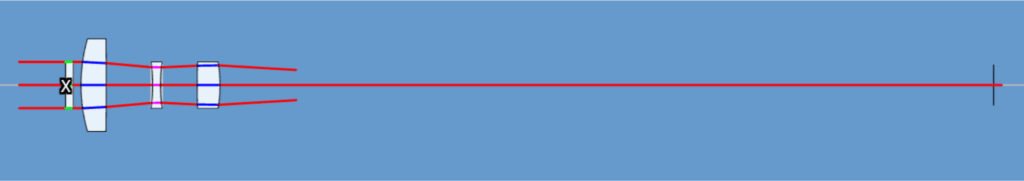
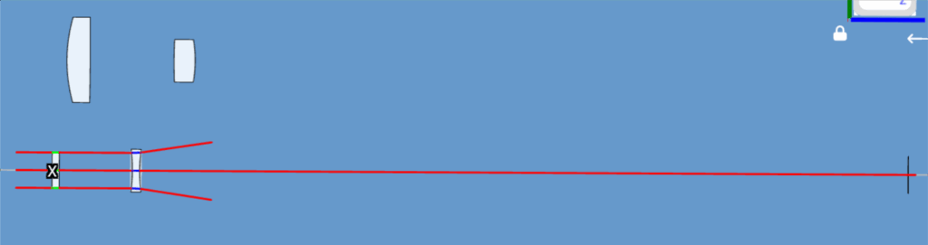
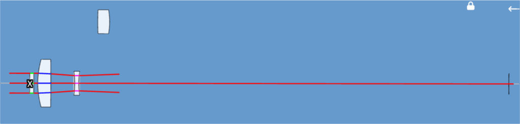
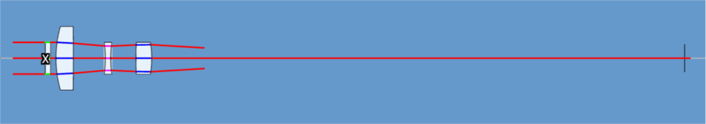
The Ritchey-Common (RC) test is a widely used optical method for testing large plane mirrors, initially proposed by A. A. Common in 1888 and detailed by G. H. Ritchey in 1904. The RC test extends the Foucault test for spherical surfaces by placing a flat mirror in the path of a diverging beam reflected off a spherical mirror. If the reference sphere is perfect, the setup is auto-stigmatic, perfectly imaging a point source back on itself. Residual power in the flat introduces some astigmatism too. Today the RC test is often done using interferometry, positioning the point source at the reference sphere’s center of curvature. This approach generates interferograms that require specific data reduction techniques due to the unique setup where light does not strike the test piece at normal incidence. See figure #1 below for RC typical setup.

Figure #1: Ritchey-Common (RC) test configuration

The source setup creates an outgoing spherical diverging beam to be reflected by the surface under test and the reference spherical mirror, resulting in an incoming (return) converging beam. The source is positioned at the center of curvature (CC) of the spherical mirror, which acts as a reference. In the simple case where the surface under test is flat, the return incoming beam is imaged at the spherical mirror’s CC, or near it.

In the context of interferometry, a transmission sphere can be used to create the outgoing beam, which eventually interferes with the incoming beam reflected back from the spherical mirror and the surface under test. This setup constitutes a double-pass test. The angle theta, known as Ritchey’s angle, is critical in this setup. The combination of the diverging nature of the outgoing beam and the angle theta (typically not zero in the RC test) creates a specific non-linear mapping between the profile of the surface under test and the wavefront of the incoming beam. This mapping is a crucial aspect of the RC test and similar tests. Data reduction is necessary to relate the measured wavefront (obtained from an interferometer, a wavefront sensor, or using image space phase retrieval or phase diversity methods) to the optical surface deformation (profile) under test. Several mappings have been developed to address this issue, such as those proposed by T. A. Fritz (see “Interferometric Evaluation for a Ritchey-Common Test Configuration,” M.S. Thesis, U. Arizona, Tucson, 1980). In this document, we propose a method to directly retrieve the surface profile from the image formed by the incoming beam using AI. This is related to Innovations Foresight’s AI4Wave technology, which has been used for phase retrieval (U.S. Patent 11,300,445 – System and Method for Wavefront Sensing with Engineered Images). Here, the RC test is used as an example of a possible implementation of such an approach, but it is not a limitation. Also, this approach can be implemented in reflection, transmission, or a combination of both. For instance, it can be used to measure both sides of a transparent surface, including its thickness.

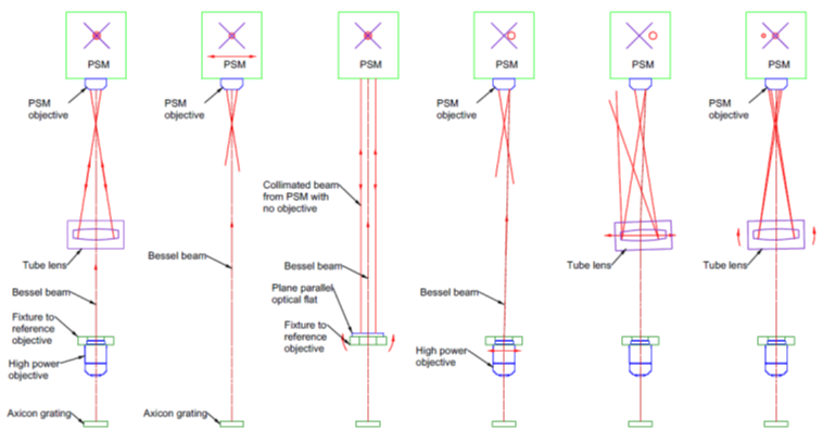
Using RC test mapping formulas (exact or approximated) or ray tracing techniques, one can compute the return incoming beam and its wavefront for a given profile of the surface under test. By applying scalar diffraction theory, one can then compute the image formed by the incoming beam at or near the spherical mirror CC. In the context of phase retrieval, we typically use a defocused image, either intra or extra-focal, though other phase modulations can also be used. The general idea disclosed here is to use such an image to directly retrieve the surface profile without having to map it from the wavefront, not even needing to know the wavefront. However we can also retrieve the wavefront if needed. One interesting aspect of using image space wavefront sensing (also known as phase retrieval when using a single image and phase diversity if one uses several images at different defocus positions) is that for weak incoming return beams, we do not face, nor need to deal with, any intensity mismatch between the incoming and outgoing (reference) beams, as we would with interferometry. This issue can be quite challenging if the surface is uncoated (clear) since the return beam could exhibit very low intensity. In the context of image space wavefront sensing, there is no interference, and we can always improve the signal-to-noise ratio (SNR) by increasing the exposure time of the camera capturing the image of the incoming beam. Also, since there is no interference, by nature this approach is very robust against vibration and other artefacts.

For simplicity, let’s assume the surface under test is circular, and its deviation from a perfect flat surface is described by a set of Zernike polynomials and their coefficients. This is not a limitation of the method; other shapes can also be used. Additionally, other methods for describing surface deviation from flatness can be employed besides Zernike polynomials. For instance, one could sample the surface at specific known locations instead of using the Zernike parametric description. We could also combine the Zernike polynomial parametric surface departure description with other methods. In the context of a circular surface and using Zernike polynomials, we can compute the incoming wavefront error due to the surface under test using ray tracing, for instance. This calculation uses the Zernike polynomials related to the surface under test and the knowledge of the test setup (theta angle, spherical mirror, including its own surface error, as well as the entire test system geometry). In short, this means that the wavefront error WF(u,v) of the incoming beam at some location along the return path after the second reflection from the surface under test is a function of the surface S(x,y) departure (error) from a flat surface. Here, x and y refer to the 2D position on the surface under test, and u and v to the 2D position on the wavefront error measured on a plane orthogonal to the return beam path at some location z along it. We have:

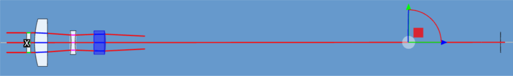
WF(u,v,z) = fmap(S(x,y))

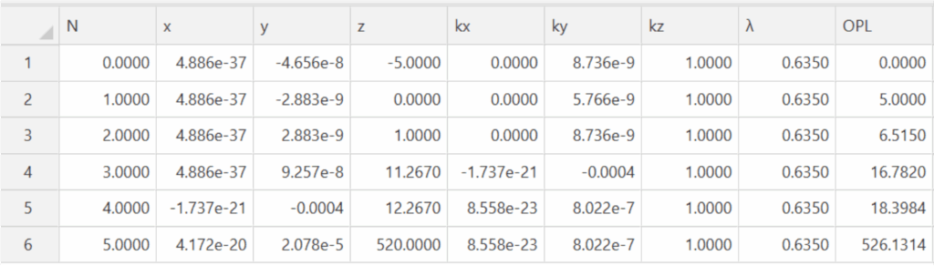
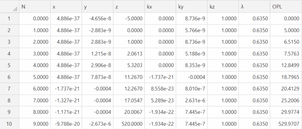
fmap is the function relating the surface errors to the wavefront error (departure between a perfect spherical wavefront and the actual wavefront). As mentioned before, for image space phase retrieval, one typically uses a defocused image (this is not a limitation of the method here other phase modulation could be used) either before the mirror CC or after the mirror CC. By choosing the z value to be close to the spherical mirror CC with some known defocus modulation (some distance away from CC), we can compute the wavefront of the incoming (return) beam using exact ray tracing calculations (or some mapping functions) and then the diffraction pattern using the Fourier transform of the WF. The WF is obviously limited in extension by the surface under test diameter d or by the spherical mirror diameter D. One of them acts as a stop in the system. In the most common situation, the surface acts as a stop, which means that the WF is defined (non-zero) inside an elliptical-like shape (resulting from the mapping of the circular surface for a given theta angle, spherical mirror radius, and diameter D). The figure #2 below shows both cases with a system stop defined by the circular surface under test or by the spherical mirror. We can clearly see that when the circular surface under test (circular is just an example, not a limitation) is the system’s stop, the resulting defocused image is elliptical in nature. Its exact shape is more complex than an ellipse because the surface stops a divergent spherical beam. When a circular stop is placed in front of the spherical mirror, becoming the system’s stop, as expected, we now have a round (circular) defocused image. The shape of the defocused image does not matter for the description of this method. When creating the samples for the training, validation, and testing databases for the neural network (or any machine learning and function approximation tools) used by AI to learn the inverse function relating the defocused image to the Zernike polynomial coefficients (or other ways to describe the surface under test error/shape), we will automatically account for any shape of the defocused image and therefore the surface under test. It should be understood that using mapping functions or ray tracing, we can express the return (incoming) beam phase error relative to a perfect spherical wavefront (if there is no aberration and a perfectly flat surface).

We can also express the magnitude of the return beam, basically the region where it is non-zero (here we assume that we have uniform illumination of the surface under test, yet this is not a limitation; we could handle any beam shape, like a Gaussian beam as well). This will define the pupil shape (circular, elliptical, or any other shape, including obstructions, if any) used to compute the diffracted defocused image through the 2D Fourier transform, as discussed above. It should be understood that using the Fourier transform is a convenient way to compute the diffraction pattern (typically a defocused image), but other techniques can be used, especially in the context of large angles where we cannot assume sin(x) ≈ x (small angle approximation) and similar approximations. We are also not limited to scalar diffraction theory; although it is the most common approach in most applications, it is not a limitation of this method. All we need is to compute sufficiently accurate defocused images (including noise and artifacts, if any) to be able to compute the inverse function through machine learning (function approximation) relating the image to the surface under test to some level of accuracy.

Figure #2: RC test defocused shape versus system’s stop location (theta = 90 degrees)

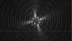
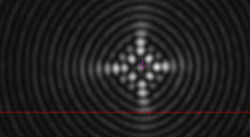
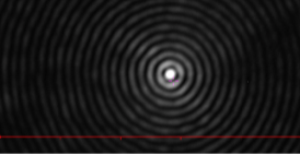
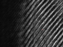
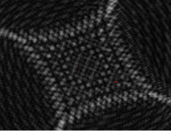
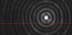
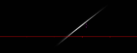
In Figure 2, the sensor is placed behind the source on axis for simplicity. In practical implementation, one can use a beam splitter in front of the source to separate the outgoing and incoming beams, or slightly tilt the surface, or the mirror or the source, or use a combination of these methods to offset the return image from the source. This can be done with minimal aberrations, which, if present, can be subtracted after proper calibration. The next figure #3 shows some examples of defocused images for some basic deformations of a flat circular surface described by the Zernike polynomials. Here theta, the Ritchey’s angle, has been set to 30 degrees and the outgoing beam at f/2. The circular surface under test is the system’s stop.

Figure #3: RC test surface error 2D heat plot, related defocused images, and wavefront 2D heat plots. Theta = 30°, beam at f/2. Surface departure expressed using circular Zernike polynomials, all values in wave RMS.

As discussed above, using ray tracing or other mapping functions, we compute the return (incoming) beam wavefront and then the related defocused images (typically using the Fourier transform) for a given surface departure (from flat). This departure can be conveniently expressed with the Zernike polynomials (but this is not a limitation). By selecting a defocus bias (in this example, 3 wave RMS), we create the necessary phase modulation to ensure the
uniqueness of the solution, meaning there is a unique image related to a unique wavefront and
therefore to a unique surface departure (deformation). This ensures convergence to an accurate
solution during the training of the neural network or equivalent function approximation tool.
We typically build a training, validation, and test database with only simulated images; we do
not need actual images for this method (although we could use some or mix synthetic images
with actual ones if we choose). Pure simulations using the above mathematics allow for the
creation of many samples (many millions) in order to sample well the inverse function for a set
of Zernike polynomials and related coefficients used to describe the surface departure (or other
methods). This is essentially identical to the approach used in Innovations Foresight’s AI4Wave
technology. Here, we reconstruct the surface instead of the wavefront from the image (we could
do both as well). This is a direct approach that does not need to solve any non-linear problems or
equivalents at run time. Once the training of the neural network has been done and validated, the
calculation of the surface departure (the Zernike coefficients or similar) from a given defocused
image is extremely fast, taking only a few milliseconds on most simple PCs. Another important
point to mention is that since there is no run-time optimization, we do not have to deal with local
minima and good enough initial guesses. All the performance, accuracy, and bias were already
validated during the training of the neural network, or any relevant function approximation
algorithms. This validation of the performance can be done with as many samples as we may
want since we can compute them.

Figure #4: Synopsis of training the inverse function relating defocused images to surface
departure from flat, using Zernike polynomials.

So far, we have considered the RC test to measure the reflection of a flat surface. However, the
same concept can be used to measure both the surface and the thickness, as well as the wedge, of
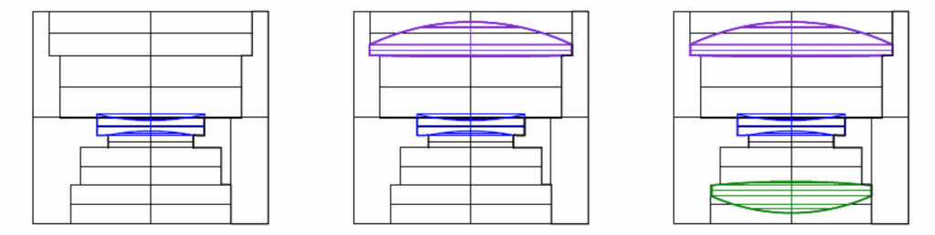
both sides of an opaque (yet reflective) surface or, more interestingly, a transparent flat window of any shape. For simplicity, we are considering a circular window, but this is not a limitation. The simplest approach would be to use two RC tests based on the specular reflection of the window, as shown in Figure #5 below (with theta set at 45 degrees for convenience). The first spherical outgoing beam is depicted in red, while the second is in green.

Figure #5: Double-Sided Reflecting RCT Test

One drawback of this approach is the need for two reference spherical mirrors and sources. In the context of a transparent flat window under test, there is the option to use a reflective and transmissive test. The former is a classic RC test, while the latter is a modified version of the RC test. Figure #6 below shows the concept (with theta set at 45 degrees for convenience). The reflected rays are depicted in red, while the transmitted rays are in green. However, for both sources (RC test on reflection, red rays, and on transmission, green rays), we observe both reflections and transmissions on each sensor. There is only a single reference spherical mirror.

Figure #6: Flat window measurement using RC test in reflection (red rays) and transmission (green rays). Each sensor captures two primary images: one from the reflection source and one from the transmission source. Flat window’s internal reflections not considered here.

Each sensor—one for the reflection RC test side and one for the transmission RC test side—exhibits two defocused images with the same shape (system’s stop at the level of the flat window). These are the primary reflection and transmission images. For simplicity, we consider the thickness of the flat window to be infinitely small, so there are no internal reflections. Figure #7 shows the internal reflections for an on-axis ray from the reflection RC test source (on the left). These reflections also occur for the transmission RC test. They can be addressed by using a spacial filter near the mirror CCs if there is any overlap between the defocused images and their internal reflections. Such a filter is essentially a circular hole of the proper size to allow the primary incoming beams (reflection and transmission) to pass through while blocking the reflections. The latter are separated by some distance (translation) related to theta, the window thickness, and its index of refraction. In this document, we won’t consider such reflections since they can be filtered out or ignored by cropping the proper subframe on each sensor. However, we mention them here because they can also be conveniently used to gather more information about the flat window under test if necessary. For instance, the translation distance of such internal reflection images tells us about the window thickness, among other things. It should be understood by anyone skilled in the art of engineering that we could process such images from these reflections in the same manner using AI, or equivalent tools, to retrieve information about the flat window’s surfaces, thickness, and wedge angle. This may improve accuracy and SNR, for instance. Those reflections can be combined with the primary image or not depending on the context.

Figure #7: Some internal reflections from the flat window under test. The spherical mirror (which should be located at the bottom of this figure) has been omitted for simplicity. The incoming rays are therefore not considered here.

In the context of the RC test in reflection and transmission depicted in Figure #6 above, we notice that we have reflection and transmission information even with a single source. The decision to use one or two sources depends on the nature of the information we want to retrieve and the nature of the surface under test. In short, we could use a single source (either the reflection or transmission one) if there is no ambiguity in the wavefront reconstruction when using the defocused image, or images, and therefore no ambiguity in the information we are looking for, such as surface departure from flatness, thickness, or wedge. We could also use a single sensor with a single source or any combination of those (one/two sources, one/two sensors). The final decision is related to the above question of the uniqueness of the solution for the inverse problem, known information on the surfaces, constraints, as well as SNR and test geometry. Therefore, it should be understood that even if we describe a system with two sources and two sensors, this is not a limitation of the method but rather a general description using some implementation (embodiment).

When having more than one image (from one or more sensor, or over time, or from several wavelengths, or a combination), data fusion for the artificial neural network (ANN) or a similar function approximation tool can be done in different ways, including using one or multiple ANNs. In one embodiment, a unique composite image features several defocused images from one or two sensors, or more and one or two sources, or more, or over time, or over wavelengths (including all combinations). This composite image is provided to the ANN for calculating the characteristics of the surface under test, like depicted in figure #4. Among the outputs, but not limited to, will be the first side surface departure or equivalent from flatness or any expected profile or just the absolute profile. This can be done, for instance, using the Zernike polynomials as in figure #4, but this is merely an example, not a limitation. Other information could include the second (other) side surface departure from flatness or any expected profile or just the absolute profile. We may also want to extract the surface under test thickness and any wedge. Other information may be extracted, such as surface index of refraction, material index of refraction, or several indices of refraction in the surface is made of various material or gradient of index of refraction as well as the optical extinction in the context of a somewhat transparent window. We may also want to know the surface polarization effect in terms of reflection and/or transmission. The existence of surface defects (localized high spatial frequencies, defects, or structures) as well as any internal defects or scattering properties may also be estimated from the composite image. We describe in the document monochromatic illumination implementations, but this is not a limitation either. We could have several wavelengths or a broad spectrum or a combination of any sources. We could also have other sources located at different positions with other sensors; the typical configuration of two sources presented here is not a limitation either. In the context of several ANNs, we could feed one from the output of another or provide several separate images to a given ANN instead of a single composite image. Any combination of these is possible depending on the problem and expected performance. It is also possible to use ANN or equivalent as time series to process images and/or data from iterations. One possible implementation could be similar to transformers used in language models. All the above implementations, combinations, and permutations are understood to be well known by anyone skilled in the art of machine learning and optimization.


In some situations, we may want, with the same system, to measure both the entire surface under test as described in the above example and discussion or to measure a smaller area of the surface on either side. In this context, we describe a novel approach using a movable stop of some shape conveniently designed to measure some defined area shape (like a disk, a rectangle, an ellipse, or any other shape) of the surface under test. The stop could be made of several non-adjacent holes too; it is not limited to a single one, whatever its shape. Such a stop may be moved to measure or scan the surface at several locations, with or without overlaps. The stop could have a variable shape and/or size too. A convenient location for such a stop, but not a limitation, is to place it in front of the reference spherical mirror. We could also have several stops combined with several spherical mirrors.

Figure #8 below shows an implementation, as an example, in the context of the RC test combining reflection and transmission as depicted in figure #6. Here the stop is placed in front of the unique reference spherical mirror. It is understood that the stop can be moved freely in any direction (3D) and its shape changed as well. Figure #8 is just an example, not a limitation, of such an implementation. The number of sources, mirrors, sensors, and stops, their shapes and positions, as well as the wavelengths in use, can all be tailored for a given goal.


One very interesting feature of having a movable, or/and changing shape, stop is the ability to combine full-surface measurements, or several image with different stop configurations and locations, or both, with local data from image taken with a stop in place (smaller aera in the surface under test). This allows the separation of any defocus errors seen by the image (or interferograms or any other means) from the RC test setup versus any power (quadratic departure) from the surface under test. In a normal RC test, we need to take at least two data sets (images, or interferogram, or others) in different configurations, for instance, by rotating the surface under test or changing the angle theta, or both, to separate any defocus observed in the image between the surface under test contribution and the setup defocus error contribution.

The moving stop provides a very convenient way to solve this issue without moving anything else but the stop or just changing the stop shape, or both. This offers a valuable advantage in terms of accuracy and speed. A small stop also allows retrieving high spatial frequency properties of the surface under test, such as roughness. It should be remembered that the defocused image (or phase-modulated engineered image) carries a lot of information about the wavefront phase, and therefore the surface departure in our case, besides piston. This includes roughness as well. It is understood that the images from the moving stop can be processed in the same way as the full surface images. Combining full images and/or stitching the images from the moving stop are options as well. We could equip the stop with some optics or CGH in some configurations. We could also use a mask instead of a simple stop near the reference spherical mirror (or elsewhere in the system, or several masks) for performing sparse aperture imaging and interferometry (like a Hartmann’s mask, for example) and/or as a coded aperture. Such a mask, or masks, could be moved and/or changed over time.

Finally, in this document, we have omitted some auxiliary optics that can be used for magnification of the image for a given camera and sensor pixel size, or to perform wavelength and/or spatial filtering. These include the possibility to correct for coma and astigmatism in the context of a diverging spherical wave passing through a transparent flat surface (a window). We could use such optics to cancel these known aberrations for the nominal, expected thickness, wedge and index of refraction of the window so that the image will only carry departures from those values and the surface itself. Total or partial cancelation of the wavefront errors due to the system optical aberrations and/or the transmission through the flat window can be done in many ways, including by using computer-generated holograms (CGH). All possible auxiliary optics are well known to anyone skilled in the art of optics.

Figure #8: RC test with a moving stop in front of the spherical mirror. The defocused images exhibit a circular shape since the stop acts as the system stop now.

Chapter 23 Alignment of Convex Surfaces

This chapter may seem out of sequence, but it tackles a recurring challenge that arguably deserved attention in a previous chapter: aligning convex surfaces. These surfaces appear nearly as often as their easier-to-align concave counterparts, yet they’re frequently overlooked—perhaps because they’re more difficult to visualize and work with. But they do exist, and they can’t be ignored. So, let’s dive in.

If a convex surface has a short radius of curvature—say, less than 10 mm—it’s usually within the working distance of most microscope objectives. For instance, a common Nikon 50× objective has an 11 mm working distance, making it easy to align a 10 mm radius surface to within a fraction of a micron. Several manufacturers also offer long working distance objectives; for magnifications up to 10× (and sometimes higher), these can reach a working distance of around 35 mm. The trade-off? They’re noticeably bulkier than their short-working-distance counterparts.

If you need more than about 35 mm of working distance, a simple trick is to use a common plano-concave lens or an achromatic doublet with a focal length longer than the surface’s radius of curvature instead of a microscope objective. Since you’re using the lens on-axis and with monochromatic light, any minor aberrations will be symmetrical, and centroiding algorithms handle symmetrical images very well. The trade-off is a reduction in both lateral and axial alignment sensitivity, proportional to the ratio of the tube lens focal length to that of the objective. In many cases, though, this loss is negligible.

If you’re worried about losing sensitivity, there’s another way to extend the working distance—up to what I’d call a practical limit of 100–150 mm. Use a standard 10× objective on the PSM (or any other centering instrument) and add a 1:1 relay with an object distance in the 100-150 mm range. The catch is that you now have a lens system cantilevered out in front of the PSM, which is both vulnerable to damage if bumped and, frankly, looks a bit odd. Still, it gives you that extra working distance without sacrificing the 10× objective’s sensitivity.

Longer radii

Of course, this still doesn’t cover every practical case. The fix isn’t all that different from the 1:1 relay just discussed—you need an auxiliary lens to transform the diverging reflection from the convex surface into a converging one. To preserve sensitivity, the auxiliary lens should also be used with 1:1 conjugates. This puts a practical upper limit on the surface radius—perhaps 500 to 1000 mm—depending on the size of your optical table. For example, if you’re aligning a 1 m radius convex surface, a good choice would be a biconvex lens with an effective focal length (EFL) of 500 mm, giving you object and image distances of about 1 m each.

The first objection you’ll probably hear when suggesting this approach is something like, “But the surface we’re aligning is 100 mm in diameter—a lens that size would have to be custom-made and ridiculously expensive.” Your counter: “No need. I’ll use a 25 mm diameter catalog lens.” The pushback then becomes, “But that won’t cover the whole aperture.” This is where you explain that alignment is a first-order optical problem: if the central 25 mm of the surface is aligned to within 1 second of arc, the entire surface is aligned to that same precision. That’s because in first-order optics, small tilts or shifts measured in the central region translate directly to the same angular accuracy across the whole surface.

Once they’ve conceded that point, the next question is, “Okay, but how are you going to align this auxiliary lens?” That’s when you head to the whiteboard and sketch out the setup—see Fig. 1a. The drawing shows all the components and their final positions needed to align the convex surface (shown in green).

Fig. 1 Steps for aligning a convex surface using a ball reference

The first step in the alignment process—shown in Fig. 1b—is to place a specular ball so that its center sits at the intended center of curvature of the convex surface. Next (Fig. 1c), insert the biconvex lens and illuminate it using the PSM’s point source. Place a white card to the left of the biconvex lens to see where the light comes to focus. Adjust both the lens and the PSM until the object and image distances are roughly equal, and the focused spot lands on the surface of the ball. At this point, you should see a cat’s-eye reflection from the ball, centered on the PSM crosshair. Aim to center the focused spot on the ball’s surface as precisely as possible—the out-of-focus cat’s-eye will appear football-shaped unless you’re well aligned. (If you’re not well centered on the ball surface, finding the center-of-curvature reflection in the next step will be much harder.)

Next, move the PSM slightly closer to the lens, increasing the image distance so the focused spot lands at the ball’s center. You’ll see a defocused return from the ball’s center of curvature that isn’t yet on the crosshair. Make small, careful adjustments until that reflected spot is both sharply focused and centered on the crosshair. Once you’ve achieved this, the biconvex auxiliary lens is correctly positioned for aligning the convex surface—because the surface’s center of curvature now coincides with the center of the ball.

Now insert the convex surface and look for its focused reflected spot near the PSM’s outgoing focused spot. A white card placed in the path of the outgoing light makes it easier to spot the reflection. Adjust the convex mirror until the reflected spot returns into the objective and you see the image on the PSM monitor. It’s easier to start with a low-power objective to locate the spot and then switch to a higher-power objective for the final fine-tuning.

Figure 1 isn’t to scale—the proportions don’t reflect the reality of 1 m object and image distances with a 25 mm diameter biconvex auxiliary lens—but it does illustrate the principle of aligning a convex surface. An easier to initially align variation of the procedure is to replace the ball in the final step with a concave spherical mirror. At first, this might seem like a more complicated setup, but in practice it’s easier—because the mirror’s reflection is much easier to locate than the ball’s, especially as the object and image distances increase. For this version, see Figure 2.

Fig. 2 Alternative method of aligning a convex surface when object and image distances are long

The procedure begins the same way as before—using a ball to define the location of the convex surface’s center of curvature. The PSM is focused on the center of the ball, making its focus coincide in all three degrees of freedom with the desired center of curvature. Then the ball is removed, and a concave spherical mirror—typically with a radius of 50 to 100 mm—is inserted and aligned so that its own center of curvature matches the PSM focus. For long object and image distances—meaning slow, low-NA light cones—it’s far easier to detect the return reflection from the concave mirror than from the short-radius ball. That’s why this approach, despite looking more elaborate, is actually easier and faster in practice.

With the concave mirror in place, insert the biconvex lens and position the PSM at its far conjugate. Using a white card, adjust the PSM so the lens forms an image of the PSM focus near the intended center of curvature of the convex surface. Use the card to help center the reflected spot from the mirror on top of the incident spot by moving the PSM. Once these spots are roughly aligned the focused image at the PSM focus should now be easy to see. Continue adjusting the PSM until the reflected spot is both centered and sharply focused on the crosshair, while keeping the lens’ object and image distances roughly equal.

Once the combination of the concave mirror, lens and PSM is finished, the convex surface is inserted just as in the case of using the ball. The convex surface is adjusted in 3 degrees of freedom until the reflection from its surface is centered on the PSM crosshair. 

Although Fig. 3 may be a bit hard to interpret, it shows real hardware set up to use the ball method for aligning the convex side of a meniscus lens. An auxiliary lens was used so that the convex surface’s center of curvature lay on the center of a ball positioned midway between the meniscus and the nearer ball. The concave side of the meniscus was aligned to the ball closest to the PSM. This setup used two PSMs so that both centers of curvature could be observed at the same time—because seeing both simultaneously makes it possible to align the meniscus in both tilt and decenter in a single process.

Fig. 3 Alignment of a meniscus lens using an auxiliary lens to view the convex surface

Very long radii

When the radius of the convex surface exceeds about 1 m, it’s time to switch methods entirely. Over the PSM’s 8 mm aperture (with the objective removed so it can function as an autocollimator) a 1 m radius surface has a sag of y2/2R = 16/2000 = 8 µm, giving the surface an effective object distance of about 500 mm. With the PSM’s 100 mm EFL tube lens, this causes the image to form at 125 mm instead of at 100 mm for a collimated wavefront. The result is a 2 mm diameter image at the camera. Because the image is rotationally symmetric, the centroiding algorithm doesn’t care about its size, it simply finds the center of the intensity pattern. In fact, it can do so even more precisely, because now there are roughly 264,000 pixels to centroid on instead of just 10–20 for a sharply focused spot from a plane wavefront. For convex surfaces with radii of 1 m or more, it’s best to use the PSM as an autocollimator and centroid on this out-of-focus image.

Conclusions 

There are at least two key take-aways from this discussion of convex surface alignment. First, there’s no “one-size-fits-all” approach to optical testing—you must look at the first-order geometry of your setup to decide what’s both practical and sensitive enough to get the job done. Second, while you can center a convex optic accurately over a wide range of radii if you choose the right method, judging axial distances or best focus becomes tricky when working with small-diameter optics and long radii. The problem is that the numerical aperture of the light cone is too small, and the depth of focus is proportional to the square of the NA. In the next chapter, we’ll explore ways to tackle this challenge and improve focus detection for long-radius surfaces with low-NA light cones.

Chapter 22 – Simulation of the alignment of a Cooke triplet using a Bessel beam reference

For some time, I wanted to simulate the assembly of a Cooke triplet using a Bessel beam as a reference,
and assuming the hardware constrained the alignment of each element to either a tilt or decenter as is
the case for many precision lens assemblies. A new optical design software is now available that makes
this modelling relatively easy whereas I was struggling before. What I discuss here was done in about 2
hours using KostaCloud, https://kostacloud.com, a software that has many features that make this sort
of modelling easy.
Fig. 1 shows the order of assembly in a typical cell where the central element must be inserted first
because of its small diameter. Because the surfaces are concave, these type elements generally have a
plane annulus ground on both sides that sit against the seat and a retaining ring. I have assumed that
this element has a 1 mradian tilt error in the ground surface so the optical axis of the lens is tilted about
3 minutes of arc, a maximum typical centering tolerance for catalog optics.


Fig. 1 Assembly steps for a Cooke triplet in a cell where the central element is inserted first
The assembly layout is shown in Fig. 2 and Table 1 is the lens design.


Fig 2 Assembly layout with a Bessel beam detector 100 mm from the lens


Table 1 Cooke triplet design including a dummy stop element and a detector plane


The plano first element in the design looks odd, but this is to get around a design feature where the stop
is the reference element in the design, and if the element with the stop moves so does the reference
frame and this is what we want to avoid during alignment. Putting the stop on the first surface of the
dummy element assures a fixed global coordinate system origin (the X) without impacting the design in
any other way. On the right of Fig. 2 is a detector plane (black line) that is the focus of a PSM prealigned
to a Bessel beam coming from the left.
The negative element is inserted in the cell with its 1 mradian tilt but perfectly centered. The tilt
introduces a deviation in the gut ray so that the ray is decentered 1.6 µm when it gets to the detector as
shown in Table 2, the ray trace of the system with just the central element.


Table 2 Ray trace through the dummy surface and central element (lines 4-5)


As seen in Table 2, the first and last elements of the triplet are missing. A feature of the KostaCloud
software is that you can drag elements out of the beam and then snap them back in, element by
element for each step of the assembly. This makes it easy for modelling an assembly as you can see what
happens as each element is added as in Fig. 3.


Fig. 3 Alignment configuration used to create the ray trace in Table 2


If the central element is decentered +254 nm the gut ray is centered on the detector to better than 36
nm as seen in line 6 of Table 3. The residual ray angle is now about 4 µradians instead of 19 µradians.


Table 3 Ray trace after decentering the central element 254 nm


When the first element is inserted perfectly centered to the design it will have no effect on the gut ray
because the ray is perfectly centered on the element as seen in Fig. 4 and Table 4. In practice, when the
first element is inserted, it would have to be centered by sliding it over its seat or effectively rotating it
about the center of curvature of the 435 mm radius surface. The PSM can detect decenters of <1 µm and
a rotation of 0.5 µradian would cause this much decenter so the PSM sensitivity to alignment is great.


Fig. 4 Assembly after the insertion of the first element


Table 4 Ray trace after the insertion of the first element (lines 4-5)


Finally, we add the last element. In actual assembly the cell would be inverted to assemble the element.
In the design program there is no need to invert the design since the ray trace through the system will
behave similarly either way the ray goes. Fig. 5 shows the complete assembly and Table 5 the ray trace.


Fig. 5 The assembly after inserting the last element


We assume the last element goes in perfectly centered to the nominal system. However the ray coming
from the central element is slightly tilted and decentered relative to the design axis the last element will
deviate the gut ray as shown in Table 5 by 1.5 µm when it reaches the PSM at an angle of 19 µradians. To
eliminate this decentration at the PSM, the element is rotated about the center of curvature of its first
surface by 4.63 µradians to center the beam on the PSM as shown in Table 6.
The KostaCloud software makes this easy by permitting a shift of the reference point for each element to
either surface or to the center of curvature of either surface by a right click on the element as shown in
Fig. 6. The reference is returned to the initial location once the rotation is accomplished by another right
click.


Table 5 Ray trace after inserting the last element (line 8-9)


Fig. 6 Last element first surface center of curvature reference position


Once the last element is rotated so the Bessel beam is centered on the PSM we have the rays and angles
shown in Table 6.


Table 6 Ray trace after rotation of the last element about the center of curvature of its first surface


Not only is the beam centered on the PSM but the gut ray angle leaving the assembly is reduced from 19
µraduans to about 4 µradians. Also, notice the ray never deviates from the design centerline by more
than 0.4 µm nor with an angle great the 400 µradians and that is inside the central element that is tilted
1000 µradians. Otherwise, all the ray angles are single digit µradians.
All this alignment was done without ever moving the PSM from its initial position of 100 mm above the
assembled lens. While the alignment perturbations in this example may be unrealistically small in
practice, they do illustrate the sensitivity of to alignment errors and the simplicity of this method of
alignment where some degrees of alignment freedom are constrained by the hardware design.
Now that we have illustrated the method, could the assembly be done any more precisely if the PSM
were farther from the lens? We will repeat the exercise with the PSM at 500 mm from the lens.
Here is the ray trace after correcting for the tilt of the central element by decentering 307 nm in Table 7.


Table 7 Ray trace after inserting the central element with the PSM at 500 mm from the lens


The greater distance gives more sensitivity to the alignment and relative to the first case the angular
error is less, now 0.8 µradians as opposed to 3.9, roughly the same ratio as PSM distance from the lens
change.
As before, when the first element is added there is no change because the first element is perfectly
aligned. Now a 0.1 µradian rotation about the center of curvature will cause a 1 µm decenter of the
PSM, up from 0.5 µm due to the greater path.
A -5.7 µradian tilt about the first surface CoC of the last element reduces the decenter on the detector to
a few nm so there is higher sensitivity to alignment as shown in Table 8. The other significant factor is
that the residual ray angle is now 0.7 µradians as opposed to 3.9 µradians, again an improvement equal
to the increased distance.


Table 8 Ray trace data after fully aligning the Cooke triplet with the PSM 500 mm from the lens


This brief demonstration shows this method of alignment is not only simple but that the best alignment
is achieved by moving the PSM as far as possible from the lens being assembled. Not only does this give
higher sensitivity to alignment errors but keeps the metrology equipment far from the vicinity of the lens
so it is easier to accomplish the alignment. The method also opens the path to automated alignment of a
whole class of optical products.

Chapter 21 – Bessel Beam Alignment of a Single Lense

Introduction: In Chapters 14 and 15 I explained how a Bessel beam is used to align optics when you have all the necessary degrees of freedom to fully align the optics in tilt, decenter and focus. Many times, you have physical constraints due to the hardware the optics are installed in, so you don’t have the ability to both tilt and decenter the optic. The question then becomes what the best is you can do, or what is the best compromise for alignment, given the constraints. This chapter explores an example of centering a single optic to understand the choices better.

Initially I started out with a goal of trying to understand the entire assembly of the 50 mm efl Cooke triplet example in Zemax. It soon became obvious that there was a lot to learn from the centering of the very first element. The Cooke triplet example looks like Fig. 1 as shown in the KostaCloud optical design software I used.

Since the negative element is the smallest one it must be installed in the cell first. Depending on how the cell is designed, then one or the other positive elements are installed, and the cell inverted to install the remaining element. To make this a realistic example I assumed the negative element was edged to have a flat annulus on the side which would sit on the seat in the cell. Further, I assumed this flat annulus was tilted 1 milliradian (about 3 minutes of arc), a typical catalog optics tolerance for edging. It quickly turned out this little error made the resulting errors so small that it was difficult to see what was happening, so I increased the tilt to 10 mrad, about ½ a degree.

After centering the negative element, I went on to install the rear element, and it soon became obvious that to explain the whole process was going to get complex. This is why I backed off and decided to show in detail what was happening when I centered just the negative element. The other reason to keep this simple is that I want to contrast the Bessel beam method with that of using a rotary table to do the centering and this is a good example for doing that.

Centering a single optic: Fig. 2 shows just the negative element tilted 10 mrad and the optical axis as the line joining the centers of curvature of the two surfaces. Even this picture does not show all the details because the different centering conditions are so close together it is impossible to see without zooming in.

The optical axis of the tilted lens is the line joining the two centers of curvature and the axis is rotated about the 1st surface (left) of the lens. The optical axis line looks a little fuzzy because it shows the optical axis in 3 different positions depending on how we center the lens. We will discuss this below, but first I want to describe how the lens will be centered using a Bessel beam.

A Bessel beam is projected from the left in Fig. 2 along what I have called a gut ray from infinity. I am assuming a perfect cell seat that is perpendicular to the gut ray and that the lens annulus is sitting on this seat perfectly with no contamination, burrs or other disturbances to a perfect match.

I put a detector to the right of the lens to sense the Bessel beam. In my lab, I use the Point Source Microscope (PSM) as the detector, but any similar device will work. In my example I place the focus of the PSM 10, 100 and 1000 mm from the second surface of the lens, and each time center the PSM on the Bessel beam before placing the lens on the seat. When the lens is initially installed in the simulation it is perfectly centered to the gut ray but always has the 10 mrad tilt. The tilt causes the Bessel to shift and tilt as shown in Table 1.

Independent of where the detector is located, Table 1 shows the ray shift and ray angle leaving the lens remains the same as for the centered but tilted lens. However, to center the Bessel beam on the detector the amount of decenter goes from -3.2 µm to 3.131 µm at 1 m. Because the distance to the detector is greater the angular deviation is less the farther the detector is from the lens. If the detector were at infinity, the amount of decenter to center the beam on the detector would 3.8 µm, the shift of the ray going through the tilted lens. This is the same beam shift, or offset, one would expect getting from a plane parallel window of the same thickness and index.

Magnified view of Bessel beam paths: Looking at just the negative element, it is easier to see where the Bessel beam crosses the reference axis for different amounts of decenter to correct for the tilt of the lens, see Fig. 3.

Fig. 3 Zoomed section of negative element showing nodal points and Bessel beam intersections the lens optical axis

Even with this magnified view it is difficult to see what is happening without some explanation. The two vertical arcs are the lens surfaces surrounding the optical axis. The nodal points are shown inside the lens. For the lens centered so the Bessel beam is centered on the detector at 10 mm from the lens, the Bessel beam crosses, or intersects, the lens optical axis to the left of the lens’ first surface, the blue circle. When the lens is centered to make the beam centered on the detector at 100 mm, the intersection is the green circle to the left of the 1st nodal point.

When the lens centration is such that the beam is centered on the detector at 1000 mm, the Bessel beam intersection is the red circle just 3.3 um to the left the nodal point. This means that the lens is centered to within 3.3 um x 0.01 radians = 33 nm of the optical axis when the position of the Bessel beam is centered on the detector. Even at 100 mm from the lens, the optical axis is within 0.6 um at the nodal point. To see this better refer to Table 2.

Clearly, every lens with different powers and shape factors will behave slightly differently, but the trend is obvious. The results in these two Tables are combined in Table 3.

If the tilted lens is decentered to make the Bessel beam fall on the center of the detector 1000 mm away the beam exiting the lens has an angle of 3.9 µradians with respect to the optical axis and is within 33 nm of the optical axis transversely at the nodal point. For all practical purposes this is perfect alignment.

Conclusion: We have shown how to achieve perfect alignment to practical limits of precision using simple x-y motion and immediate feedback on the accuracy of alignment. The simplicity of the method opens the possibility of automating alignment. The insights gained by this example provide a direction for examining the next steps of adding the other optical elements to the lens assembly. We will look at this in the next Chapter.

Chapter 20: Aligning Off-Axis Parabolas with a Bessel Beam — It’s Much Easier

Introduction

In Chapter 18, I described aligning off-axis parabolas (OAPs) by placing the focus of a test instrument at
the OAP’s focus and autoreflecting off a plane mirror. Although I suggested some tips to ease the
process, the initial alignment—getting the reflected light back into the test device’s objective—remains
challenging.

Because I’ve found that using a Bessel beam makes lens alignment easier, I wondered if the same would
apply to OAP alignment. (Spoiler alert: it does!)

Initial Alignment

I started with an Edmund Optics 25 mm diameter, 15° OAP with a 387 mm effective focal length (EFL). I
projected a Bessel beam (BB) roughly along the optical axis toward the OAP and viewed the reflected
beam with a Point Source Microscope (PSM) about 400 mm away. The reflected beam was clearly visible
on a white card, which made it easy to position the PSM so the beam was centered on the 4x objective.
See Fig. 1.


Fig. 1 shows the initial image. The image width is about 40 µm, across a 100 µm field of view.

Why the Bessel Beam Helps Initial Alignment

Using a BB simplifies initial alignment for two main reasons:

1. Two Degrees of Freedom – You’re locating a beam-like spot instead of a focused point, so you
only need to search in two dimensions rather than three. You can find the spot anywhere along
the beam.
2. Single Pass Simplicity – The BB allows single-pass alignment rather than a more complex
double-pass process. Once the spot is in the objective, you can immediately begin minimizing
aberrations by reducing the BB pattern’s size.

Fine Alignment

The most noticeable feature of the image in Fig. 1 is its rotation relative to the test coordinate system.
It’s easier to reduce aberrations or spot size consistently if the image is squared with the axes. This is
done by translating the OAP parallel to one of the axes while applying compensating tilts to keep the
spot centered.

Fig. 2 shows the result after squaring the image.

Once the image is squared, as in Fig. 2, you can use the orthogonal axis adjustments to reduce the image
size. Large changes help determine the correct direction to minimize the image. As you progress, fine
adjustments eliminate residual misalignment as in Fig. 3.

Fig. 3 shows the final aligned image.

The Alignment Experience

I was surprised at how easy the alignment turned out to be. Here&#39;s why:

  • The reflected spot was easy to find.
  • Only two adjustments—tilt and decenter—were necessary for full alignment
  • Focus adjustments weren’t needed since the BB always appears in focus.
  • Progress was easy to monitor: the number of bright spots in the BB image decreased asalignment improved.
  • While aligning an OAP still isn’t as easy as finding the center of curvature of a sphere, it&#39;s not much
    harder.

Aligning a 90° OAP

Encouraged by the 15° OAP results, I tried aligning a more difficult 90° OAP with a shorter EFL. The setup
(shown in Fig. 4) was similar. The BB projector was aimed roughly along the OAP axis, and the PSM was
placed several focal lengths away—not near the focus.

Fig. 4 Alignment setup for 90° OAP (lower left) in an adjustable mount, a Bessel beam projector (upper
left) pointing along the OAP axis and a PSM (right) several focal lengths from the OAP.

After roughly mounting the optics, I turned on the BB source. Even when the core of the BB image was
~15 mm off-center from the 4x objective, the PSM still picked up the pattern (Fig. 5). This again
highlights the advantage of the BB: the outer rings offer clear visual cues for centering adjustments.


Fig. 5 Initial image seen by the PSM with beam Fig. 6 Initial image after centering the core on the
15 mm from the center of the objective PSM (Both pictures show the uncropped images)

Fine Alignment of the 90° OAP

The 90° OAP image was larger than the 15°, which makes sense given the lower f/# (f/2 vs. f/15). The
shape and initial misalignment were similar in both cases. After squaring the image to the adjustment
axes, fine alignment was straightforward, as seen in Fig. 7.

Fig. 7 Aligned BB image from 90° OAP

Comparing Figs. 3 and 7:

  • Both are shown at the same scale (100 µm bar).
  • The BB core in Fig. 3 is about 3× smaller than in Fig. 7.
  • Fig. 3 has ~8 rings, while Fig. 7 shows ~4—evidence of the different f/#s.This scale difference deserves further exploration in BB-based alignment.

Verifying Alignment

Of course, you shouldn’t just take my word for it. To confirm alignment, we can examine the double-
pass image at the OAP focus.

The BB projector was initially aligned to propagate normal to the grating, ensuring that the BB was
aligned with the OAP axis. Moving the PSM to the OAP’s focus, its internal point source illuminated the
OAP, and the collimated light reflected back through the BB grating.

Because of physical interference between the PSM and BB projector at close range, I had to move the
OAP slightly (see Fig. 4), then realign it.

The initial double-pass image (Fig. 8) was slightly astigmatic—about 50 µm long—suggesting ~8 µm
defocus (4 µm in single pass). A small tweak produced the near-perfect image in Fig. 9, where the image
size matches what I see when aligning to a Grade 5 ball—suggesting a wavefront error of ~1/8 to 1/10
wave.

Fig. 8 Initial double pass image at the OAP focus (Same scale as other cropped images)


Fig. 9 Double pass image from 90° OAP at scale, and zoomed in. The space in the middle of the crosshair
is 11 µm so the image is about half that, and half again for double pass.

Discussion

Aligning off-axis parabolas becomes much easier using a Bessel beam as a reference axis. Key
benefits include:

  • Ease of Beam Tracking – You can see the BB spot at almost any distance.
  • Straightforward Progression – Once the image appears on the detector, alignment is
    just a matter of tilt and decenter.
  • No Focusing Required – The BB is always in focus, so you can focus on making the image
    smaller and more symmetric.
  • Visual Feedback – The decreasing number of bright spots in the BB image gives
    immediate feedback on alignment progress.

If you’re using a PSM, you can finalize the alignment by moving it to the OAP focus and checking
the double-pass image off the BB projector’s grating. This confirms both BB and OAP
alignment—and, assuming the OAP is of good quality—produces a diffraction-limited result.

I hope this note helps those of you who have struggled with the frustrations of aligning off-axis
parabolas.


Chapter 19 – Microscope Objective to Tube Lens Alignment

The subject of this Chapter is prompted by several questions over the last couple of months concerning the alignment of tube lenses to high power microscope objectives. In most microscopes these days the objectives are designed as finite to infinite conjugate optics so there is a need for a “tube” lens to focus the object onto the eyepiece reticle plane or camera sensor array. Since the light is in collimated space between the objective and tube lens it would appear at first glance, the worst you would do with misalignment is vignette. However, when the requirement is for 50 or 100x magnification, even the slightest misalignment leads to loss in imaging performance.

Another use for high magnification microscopes is as part of an optical scanning system where the microscope is used backwards to move a well-focused spot across what would be the object plane of the microscope as used for viewing small objects. Here alignment affects not only the imaging performance but the linearity of the scan with angle of the input light beam. Schematic examples of both situations are shown in Fig. 1.

Fig. 1 Schematic of an infinite conjugate microscope used for viewing (upper), and a similar microscope used for scanning a spot over the image plane (lower)

We will frame the alignment question in terms of how the tube lens should be positioned relative to the objective in angle and lateral position. The spacing between objective and tube lens is flexible if it is within the design range of the tube lens, but 100 mm is a typical value. I find it easier to discuss examples using specific parameters so let’s use the following: the objective is nominally 100 x with an efl of 2 mm designed to work with a tube lens with a 200 mm efl placed about 100 mm from the entrance pupil of the objective.

Since the objective will serve as the reference for alignment, we must consider how its five degrees of freedom (DOF) are determined optically and mechanically. Fig. 2 shows typical mounting dimensions for one brand of objectives. The flange, a plane annulus nominally perpendicular to the objective’s optical axis controls angle in 2 DOF and the distance along the axis, 1 DOF. The thread diameter controls the objective’s position perpendicular to the axis in the remaining 2 translational DOF.

The threads are the weak point in this connection because every time you remove and reinsert an objective it moves laterally a few microns in a non-repeatable way. For ordinary viewing it doesn’t matter if the image shifts, but at 100 x with the tube lens 100 mm away a 1 um objective lateral shift causes an image shift of 100 um and an angular change of the collimated beam of almost 2 minutes of arc.

Fig. 2 A typical specification for the threaded interface of a microscope objective.

My understanding is that the threads are designed to have a little slop so that seating against the flange is definite. Given that the flange is a solid interface, this points to an approach to alignment. A plane parallel fixture with a bore and internal threads to match the objective is made parallel to an Axicon grating projecting a Bessel beam as in Fig. 3. The Figure gives all the steps to full alignment.

Fig. 3 The steps to align a tube lens with a microscope objective starting with a fully aligned system (a) to show the various required parts of the setup

Detail a) of Fig. 3 shows the completely aligned system so I can explain the various parts of the setup and their purposes. Starting at bottom is an axicon grating illuminated by a point source to produce a Bessel beam that acts as the reference axis for alignment. The beam propagates through the high magnification objective that is screwed into a fixture that provides a mechanical reference for the objective’s location. The beam continues through the tube lens where it is viewed with a Point Source Microscope (PSM). The monitor for the PSM is shown schematically with its reference crosshair. In the fully aligned condition, both the Bessel beam and a reflection from the center of curvature of a spherical surface within the tube lens are both centered on the PSM crosshair.

Detail a) makes it clear that in the first step of alignment b) the PSM must be at the correct axial distance to view the center of curvature of an element of the tube lens once it is inserted. With the PSM at the correct distance, the PSM is translated perpendicularly to the Bessel beam to center the beam on the PSM crosshair.

Next c), a fixture is added to the setup into which the objective will be mounted. The fixture is precisely parallel so the a plane parallel window or mirror set on the upper surface will be parallel to the flange against which the objective is mounted. The objective is removed from the PSM so it acts as an autocollimator and the fixture is squared to the Bessel beam and PSM by rotation. The fixture assures the objective is held so that is axis is parallel to the Bessel beam within the precision of the objective itself.

Once the fixture is adjusted, the objective is mounted in the fixture and the objective replaced on the PSM. The fixture/objective pair is translated laterally to bring the Bessel beam onto the PSM crosshair as in detail d). Here we have shown a slight misalignment of the objective and how that moves the Bessel beam centroid off the PSM crosshair in detail d). Once the Bessel beam is on the crosshair, the objective serves as the reference to which to align the tube lens. Because of the high magnification of the objective its lateral position is located to sub-micron precision. Again, the weak point in the alignment is that removing and replacing the objective in this fixture, or in the end item mount, is the lack of repeatability of the threaded interface.

With the objective set as the reference, the tube lens is inserted in the beam. Initially the lens is misaligned and the reflection from the center of curvature may miss returning in the objective. The Bessel beam may also be misaligned, but this is easy to correct because the rings in the Bessel beam show the direction to move the lens to center the core of the beam by translation as shown by the red arrows in e).

The final step in the alignment f) is to tilt the tube lens until the center of curvature is also centered on the crosshair. There may be a bit of iterative alignment to get both spots on the crosshair as the tilting may misalign the Bessel beam and vice versa. However, the procedure converges rapidly to position the tube lens to the 1 um level perpendicular to the beam and the 1 second of arc tilt range.

If your system is designed for observing, the alignment is complete. If you have a scanning system, the scan lens is aligned following the same principles since the Bessel beam is again centered on the PSM crosshair as it was before introducing either the objective or tube lens and it is propagating with the same angle. The beam is now used as the reference to move the PSM farther up to a place where it is focused at the center of curvature of a surface in the scan lens. Once the PSM is centered, the procedure is used the same way to align the scan lens.