Author: csadmin

Introduction

In Chapter 18, I described aligning off-axis parabolas (OAPs) by placing the focus of a test instrument at
the OAP’s focus and autoreflecting off a plane mirror. Although I suggested some tips to ease the
process, the initial alignment—getting the reflected light back into the test device’s objective—remains
challenging.

Because I’ve found that using a Bessel beam makes lens alignment easier, I wondered if the same would
apply to OAP alignment. (Spoiler alert: it does!)

Initial Alignment

I started with an Edmund Optics 25 mm diameter, 15° OAP with a 387 mm effective focal length (EFL). I
projected a Bessel beam (BB) roughly along the optical axis toward the OAP and viewed the reflected
beam with a Point Source Microscope (PSM) about 400 mm away. The reflected beam was clearly visible
on a white card, which made it easy to position the PSM so the beam was centered on the 4x objective.
See Fig. 1.

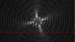
Fig. 1 shows the initial image. The image width is about 40 µm, across a 100 µm field of view.

Why the Bessel Beam Helps Initial Alignment

Using a BB simplifies initial alignment for two main reasons:

1. Two Degrees of Freedom – You’re locating a beam-like spot instead of a focused point, so you
only need to search in two dimensions rather than three. You can find the spot anywhere along
the beam.
2. Single Pass Simplicity – The BB allows single-pass alignment rather than a more complex
double-pass process. Once the spot is in the objective, you can immediately begin minimizing
aberrations by reducing the BB pattern’s size.

Fine Alignment

The most noticeable feature of the image in Fig. 1 is its rotation relative to the test coordinate system.
It’s easier to reduce aberrations or spot size consistently if the image is squared with the axes. This is
done by translating the OAP parallel to one of the axes while applying compensating tilts to keep the
spot centered.

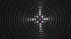
Fig. 2 shows the result after squaring the image.

Once the image is squared, as in Fig. 2, you can use the orthogonal axis adjustments to reduce the image
size. Large changes help determine the correct direction to minimize the image. As you progress, fine
adjustments eliminate residual misalignment as in Fig. 3.

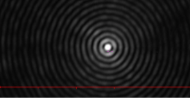
Fig. 3 shows the final aligned image.

The Alignment Experience

I was surprised at how easy the alignment turned out to be. Here's why:

• The reflected spot was easy to find.
• Only two adjustments—tilt and decenter—were necessary for full alignment
• Focus adjustments weren’t needed since the BB always appears in focus.
• Progress was easy to monitor: the number of bright spots in the BB image decreased asalignment improved.
• While aligning an OAP still isn’t as easy as finding the center of curvature of a sphere, it's not much
  harder.

Aligning a 90° OAP

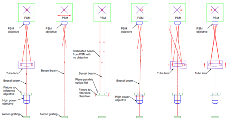
Encouraged by the 15° OAP results, I tried aligning a more difficult 90° OAP with a shorter EFL. The setup
(shown in Fig. 4) was similar. The BB projector was aimed roughly along the OAP axis, and the PSM was
placed several focal lengths away—not near the focus.

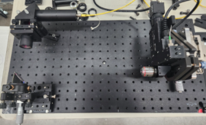
Fig. 4 Alignment setup for 90° OAP (lower left) in an adjustable mount, a Bessel beam projector (upper
left) pointing along the OAP axis and a PSM (right) several focal lengths from the OAP.

After roughly mounting the optics, I turned on the BB source. Even when the core of the BB image was
~15 mm off-center from the 4x objective, the PSM still picked up the pattern (Fig. 5). This again
highlights the advantage of the BB: the outer rings offer clear visual cues for centering adjustments.

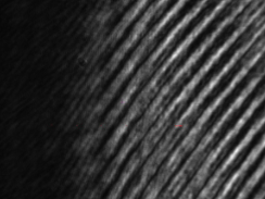
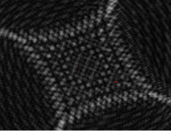
Fig. 5 Initial image seen by the PSM with beam Fig. 6 Initial image after centering the core on the
15 mm from the center of the objective PSM (Both pictures show the uncropped images)

Fine Alignment of the 90° OAP

The 90° OAP image was larger than the 15°, which makes sense given the lower f/# (f/2 vs. f/15). The
shape and initial misalignment were similar in both cases. After squaring the image to the adjustment
axes, fine alignment was straightforward, as seen in Fig. 7.

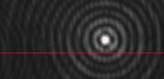
Fig. 7 Aligned BB image from 90° OAP

Comparing Figs. 3 and 7:

• Both are shown at the same scale (100 µm bar).
• The BB core in Fig. 3 is about 3× smaller than in Fig. 7.
• Fig. 3 has ~8 rings, while Fig. 7 shows ~4—evidence of the different f/#s.This scale difference deserves further exploration in BB-based alignment.

Verifying Alignment

Of course, you shouldn’t just take my word for it. To confirm alignment, we can examine the double-
pass image at the OAP focus.

The BB projector was initially aligned to propagate normal to the grating, ensuring that the BB was
aligned with the OAP axis. Moving the PSM to the OAP’s focus, its internal point source illuminated the
OAP, and the collimated light reflected back through the BB grating.

Because of physical interference between the PSM and BB projector at close range, I had to move the
OAP slightly (see Fig. 4), then realign it.

The initial double-pass image (Fig. 8) was slightly astigmatic—about 50 µm long—suggesting ~8 µm
defocus (4 µm in single pass). A small tweak produced the near-perfect image in Fig. 9, where the image
size matches what I see when aligning to a Grade 5 ball—suggesting a wavefront error of ~1/8 to 1/10
wave.

Fig. 8 Initial double pass image at the OAP focus (Same scale as other cropped images)

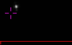
Fig. 9 Double pass image from 90° OAP at scale, and zoomed in. The space in the middle of the crosshair
is 11 µm so the image is about half that, and half again for double pass.

Discussion

Aligning off-axis parabolas becomes much easier using a Bessel beam as a reference axis. Key
benefits include:

• Ease of Beam Tracking – You can see the BB spot at almost any distance.
• Straightforward Progression – Once the image appears on the detector, alignment is
  just a matter of tilt and decenter.
• No Focusing Required – The BB is always in focus, so you can focus on making the image
  smaller and more symmetric.
• Visual Feedback – The decreasing number of bright spots in the BB image gives
  immediate feedback on alignment progress.

If you’re using a PSM, you can finalize the alignment by moving it to the OAP focus and checking
the double-pass image off the BB projector’s grating. This confirms both BB and OAP
alignment—and, assuming the OAP is of good quality—produces a diffraction-limited result.

I hope this note helps those of you who have struggled with the frustrations of aligning off-axis
parabolas.

The subject of this Chapter is prompted by several questions over the last couple of months concerning the alignment of tube lenses to high power microscope objectives. In most microscopes these days the objectives are designed as finite to infinite conjugate optics so there is a need for a “tube” lens to focus the object onto the eyepiece reticle plane or camera sensor array. Since the light is in collimated space between the objective and tube lens it would appear at first glance, the worst you would do with misalignment is vignette. However, when the requirement is for 50 or 100x magnification, even the slightest misalignment leads to loss in imaging performance.

Another use for high magnification microscopes is as part of an optical scanning system where the microscope is used backwards to move a well-focused spot across what would be the object plane of the microscope as used for viewing small objects. Here alignment affects not only the imaging performance but the linearity of the scan with angle of the input light beam. Schematic examples of both situations are shown in Fig. 1.

Fig. 1 Schematic of an infinite conjugate microscope used for viewing (upper), and a similar microscope used for scanning a spot over the image plane (lower)

We will frame the alignment question in terms of how the tube lens should be positioned relative to the objective in angle and lateral position. The spacing between objective and tube lens is flexible if it is within the design range of the tube lens, but 100 mm is a typical value. I find it easier to discuss examples using specific parameters so let’s use the following: the objective is nominally 100 x with an efl of 2 mm designed to work with a tube lens with a 200 mm efl placed about 100 mm from the entrance pupil of the objective.

Since the objective will serve as the reference for alignment, we must consider how its five degrees of freedom (DOF) are determined optically and mechanically. Fig. 2 shows typical mounting dimensions for one brand of objectives. The flange, a plane annulus nominally perpendicular to the objective’s optical axis controls angle in 2 DOF and the distance along the axis, 1 DOF. The thread diameter controls the objective’s position perpendicular to the axis in the remaining 2 translational DOF.

The threads are the weak point in this connection because every time you remove and reinsert an objective it moves laterally a few microns in a non-repeatable way. For ordinary viewing it doesn’t matter if the image shifts, but at 100 x with the tube lens 100 mm away a 1 um objective lateral shift causes an image shift of 100 um and an angular change of the collimated beam of almost 2 minutes of arc.

Fig. 2 A typical specification for the threaded interface of a microscope objective.

My understanding is that the threads are designed to have a little slop so that seating against the flange is definite. Given that the flange is a solid interface, this points to an approach to alignment. A plane parallel fixture with a bore and internal threads to match the objective is made parallel to an Axicon grating projecting a Bessel beam as in Fig. 3. The Figure gives all the steps to full alignment.

Fig. 3 The steps to align a tube lens with a microscope objective starting with a fully aligned system (a) to show the various required parts of the setup

Detail a) of Fig. 3 shows the completely aligned system so I can explain the various parts of the setup and their purposes. Starting at bottom is an axicon grating illuminated by a point source to produce a Bessel beam that acts as the reference axis for alignment. The beam propagates through the high magnification objective that is screwed into a fixture that provides a mechanical reference for the objective’s location. The beam continues through the tube lens where it is viewed with a Point Source Microscope (PSM). The monitor for the PSM is shown schematically with its reference crosshair. In the fully aligned condition, both the Bessel beam and a reflection from the center of curvature of a spherical surface within the tube lens are both centered on the PSM crosshair.

Detail a) makes it clear that in the first step of alignment b) the PSM must be at the correct axial distance to view the center of curvature of an element of the tube lens once it is inserted. With the PSM at the correct distance, the PSM is translated perpendicularly to the Bessel beam to center the beam on the PSM crosshair.

Next c), a fixture is added to the setup into which the objective will be mounted. The fixture is precisely parallel so the a plane parallel window or mirror set on the upper surface will be parallel to the flange against which the objective is mounted. The objective is removed from the PSM so it acts as an autocollimator and the fixture is squared to the Bessel beam and PSM by rotation. The fixture assures the objective is held so that is axis is parallel to the Bessel beam within the precision of the objective itself.

Once the fixture is adjusted, the objective is mounted in the fixture and the objective replaced on the PSM. The fixture/objective pair is translated laterally to bring the Bessel beam onto the PSM crosshair as in detail d). Here we have shown a slight misalignment of the objective and how that moves the Bessel beam centroid off the PSM crosshair in detail d). Once the Bessel beam is on the crosshair, the objective serves as the reference to which to align the tube lens. Because of the high magnification of the objective its lateral position is located to sub-micron precision. Again, the weak point in the alignment is that removing and replacing the objective in this fixture, or in the end item mount, is the lack of repeatability of the threaded interface.

With the objective set as the reference, the tube lens is inserted in the beam. Initially the lens is misaligned and the reflection from the center of curvature may miss returning in the objective. The Bessel beam may also be misaligned, but this is easy to correct because the rings in the Bessel beam show the direction to move the lens to center the core of the beam by translation as shown by the red arrows in e).

The final step in the alignment f) is to tilt the tube lens until the center of curvature is also centered on the crosshair. There may be a bit of iterative alignment to get both spots on the crosshair as the tilting may misalign the Bessel beam and vice versa. However, the procedure converges rapidly to position the tube lens to the 1 um level perpendicular to the beam and the 1 second of arc tilt range.

If your system is designed for observing, the alignment is complete. If you have a scanning system, the scan lens is aligned following the same principles since the Bessel beam is again centered on the PSM crosshair as it was before introducing either the objective or tube lens and it is propagating with the same angle. The beam is now used as the reference to move the PSM farther up to a place where it is focused at the center of curvature of a surface in the scan lens. Once the PSM is centered, the procedure is used the same way to align the scan lens.