Practical Optical Tabletop Alignment

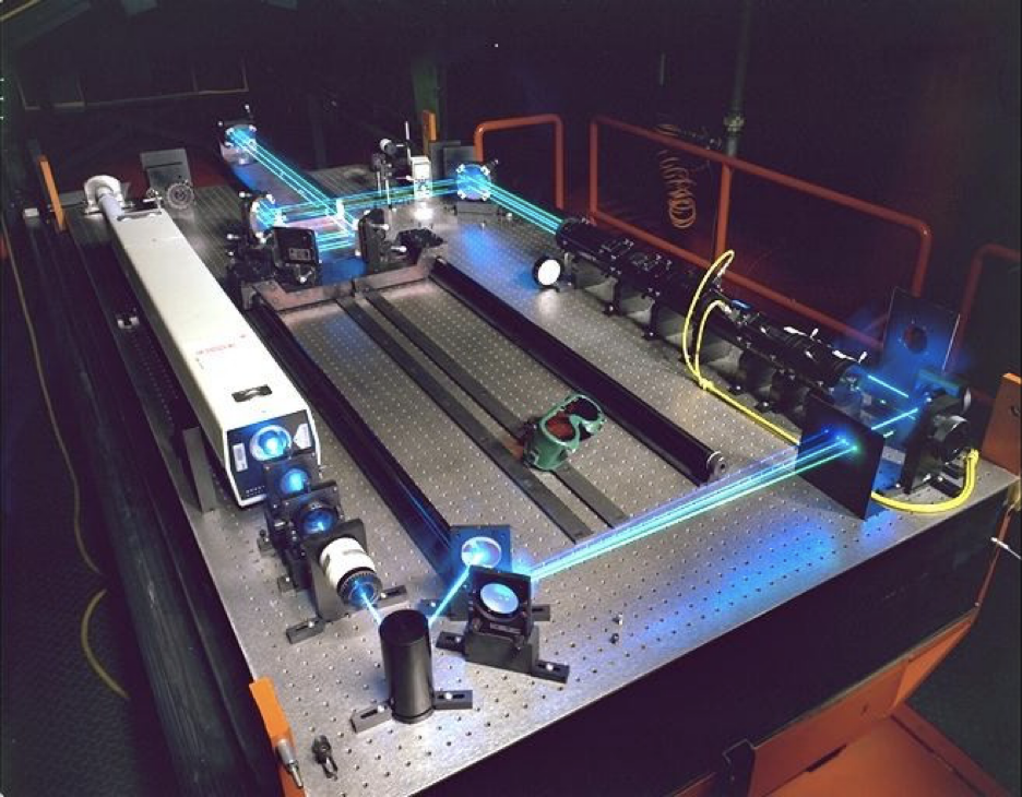
Many research projects begin as tabletop assemblies of optical components to move light from a source through an interaction zone to change the character of the light and on to a detector. The quality of the signal reaching the detector depends on the optical alignment of all the components between the source and detector. The signal quality reaching the detector often means the difference between success or failure of the experiment. In this note we discuss practical issues regarding tabletop optical alignment, like that pictured below, to realize the maximum signal quality with the minimum effort.

As a simple example, draw a line between the light source and detector to define a required system axis and use a simple positive lens as what interacts with the light in between as shown below in Fig. 1.

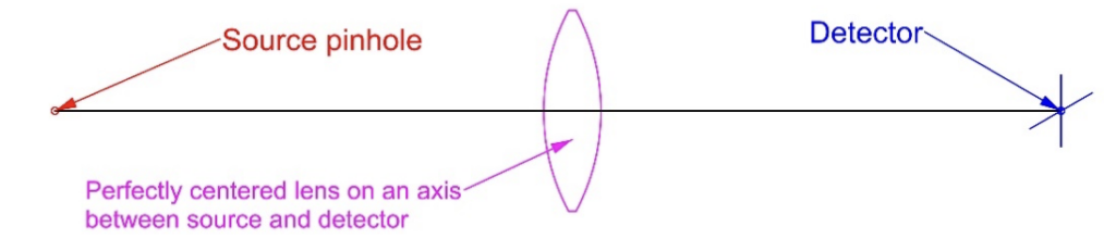
Fig. 1 A perfectly centered and tilt free lens relative to the system axis (black line) 

As each component is added between the source and detector, optimum alignment is achieved when the light path following the component is unchanged in position or angle, that is, the light reaching the detector arrives at the same location and same angle as before the component was introduced in the light path. Now we discuss how to accomplish this task.

Optical Alignment Using a Bessel beam

We [1], and others [2,3], have found that a Bessel beam propagates through optical components such as lenses and prisms as though the beam was a paraxial ray. As opposed to a real ray that comes to focus at the back focus of a lens illuminated with collimated light and is only visible as a focused spot in the back focal plane, a paraxial ray propagates an arbitrary distance. If we use a Bessel beam as our axis between source and detector, we can observe its position and direction at any point along the beam as in Fig. 2. (Details about Bessel beam creation are in the Appendix)

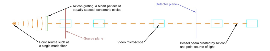
Fig. 2 Bessel beam created by a point source and Axicon grating detected anywhere along the beam

To keep the example simple, but easily extended to multiple components, assume we want to place a lens between the source and detector planes that images an illuminated pinhole source onto a target crosshair in front of a detector. We project a Bessel beam created with a point source of light on the axis of an Axicon grating down the intended path between source and detector as in Fig. 3. Beyond the detector plane we place a beamsplitter and two video microscopes at different distances from the beamsplitter. Because of the different distances we can measure any change in the Bessel beam position and direction in 4 degrees of freedom (DOF).

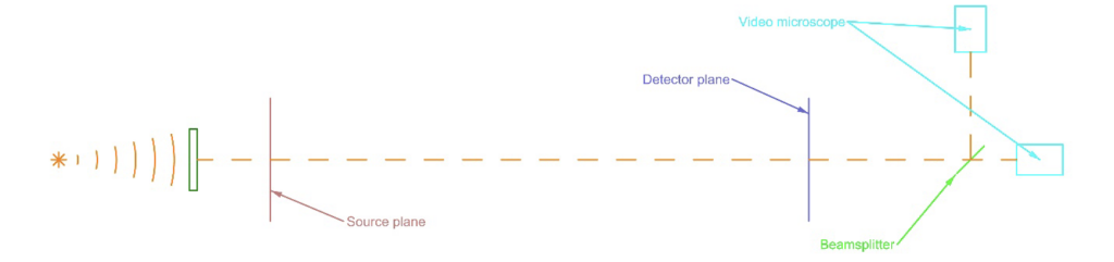
Fig. 3 The Bessel beam is deflected when a lens with tilt and decenter is inserted in the Bessel beam

Aligning a Lens in the Bessel beam

Now we insert the lens in the beam and move it in position and tilt. This causes the spots seen in the microscopes to move as in Fig. 4. There is one, and only one, position of the lens in 4 DOF for which the spots in the microscopes are centered as they were prior to inserting the lens. Now the transmitted Bessel beam is coincident with the beam before inserting the lens. This is considered perfect alignment of the lens. Since the Bessel beam is as it was before inserting the lens, it is now used as the reference for inserting the next element.

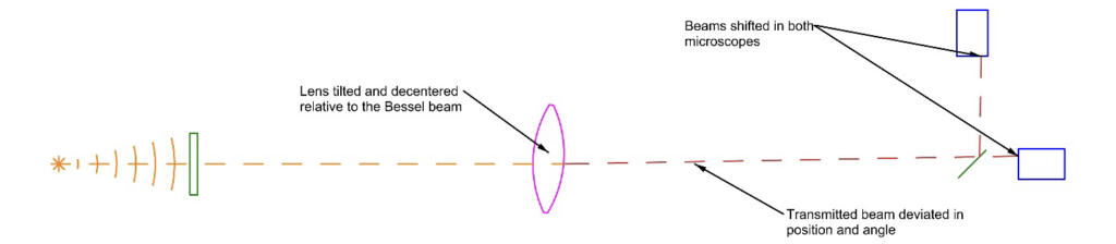
Fig. 4 Initial insertion of the lens deviates the Bessel spot location on both video microscopes

Aligning the Detector and Source to the Bessel beam

Now we must center the detector and pinhole on the reference Bessel beam. First, place the center of a reflecting ball at the design distance from the lens surface. We typically use a Grade 5, ½ inch steel ball. Have the ball rest on the end of a lens post to serve as a kinematic mount for the ball so the ball can be repeatably removed and replaced in the same position as shown in Fig. 5. Remove the beamsplitter and move in an autostigmatic microscope (ASM) so it faces the source and focuses approximately on the center of the ball. Remove the ball from the post and align the ASM with the Bessel beam. Then center the ball to the ASM using the reflection from the center of the ball. The center of the ball is centered on the Bessel beam as shown in Fig. 6. 

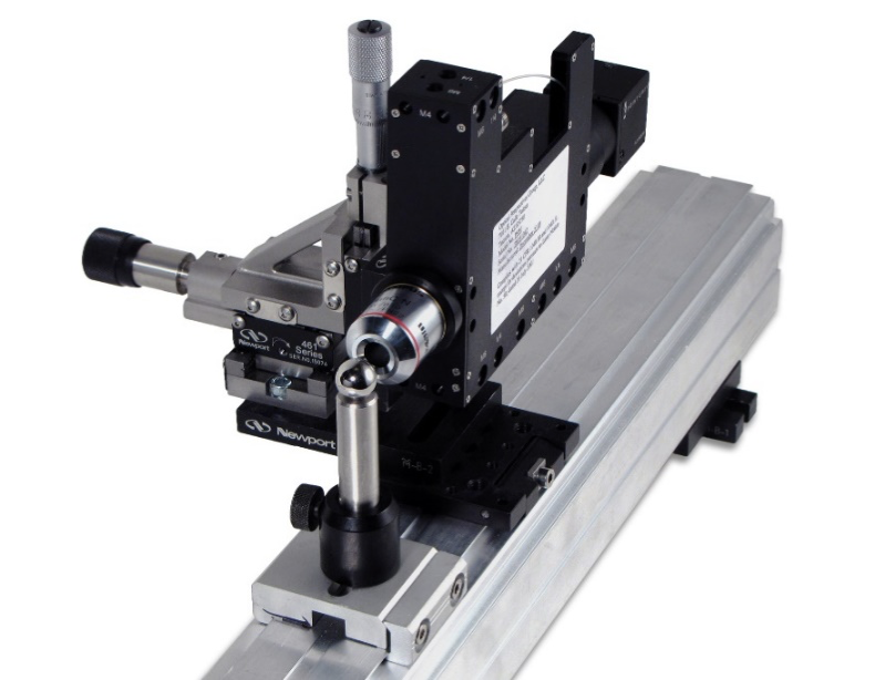
Fig. 5 Steel ball on a lens post viewed by an autostigmatic microscope focused at the ball center

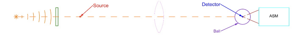
Fig. 6 The ASM is first centered on the Bessel beam and then the ball centered with the ASM

(At this point you may say I am going about this backwards, but I am doing this to explain the process. Once I finish you will realize that the Bessel beam could have been aligned with the pinhole and detector first, but it is easier to explain this way. The method works either way. Stay with me.)

Now the center of the ball is located in 3 DOF where the crosshair on the detector should go. Take the ASM away from the ball and rotate it 180° so it is centered on the ball but facing the detector. Because the ball hasn’t moved, the ASM, when centered on the ball, is focused where the crosshair on the detector should go. Remove the ball and post and insert and align the detector crosshair as in Fig. 7.

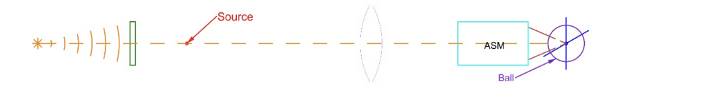
Fig. 7 The ball is used to center the ASM so the ASM can center the detector

The same procedure is used to position the source pinhole. This takes less steps because the ASM is already looking toward the source. The ASM is centered on the Bessel beam at the axial location of the source pinhole as in Fig. 8.  Now the pinhole is moved so that it is centered on the ASM crosshair. When the pinhole is illuminated it will be imaged on the detector in the correct location by the lens that is centered on the line between source and detector and is free of tilt relative to the line.

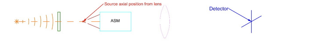
Fig. 8 The ASM is center on the Bessel beam at the axial location of the pinhole source

A Simplified Method of Alignment

This procedure seems a little complicated in that two microscopes are needed to detect both the position and tilt of the Bessel beam. A simpler method uses an additional beamsplitter and a couple plane mirrors to view the Bessel beam at two axial positions simultaneously with an ASM as in Fig. 8.

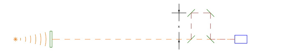
Fig. 8 Method of viewing the Bessel beam at two separate axial locations simultaneously

With this addition that views the Bessel beam at locations 2x apart, a single ASM is the only optical test instrument needed to do this alignment. The ASM is used to align the lens to the Bessel beam, and then subsequently used to align the detector and source via the use of ball data points. 

Clearly this method can be extended to multiple lenses or fold mirrors to bend the beam in any desired direction. Once the first component is centered in the beam free of tilt and decenter, the Bessel beam is coaxial with itself before the first component was inserted so that the beam. This being the case, the Bessel beam is the reference axis for the next component.

Conclusion

While we have explained a simple method of tabletop alignment, we have not said anything about the practical issues of alignment. One of the first is why not just use a laser beam for alignment. The most important answer is safety. The Bessel beam diffracts light over a wide cone angle, so the energy density is low. The bright core of the Bessel beam is smaller in diameter than a laser beam by at least a factor of 10, more typically by a 100. The laser obeys the optics of real rays while the Bessel beam behaves as a paraxial ray and gives more information about how the beam propagates through the interaction zone than a laser.

On the hardware side, everything we have described using an ASM, in this case the Point Source Microscope (PSM), could be done with a classical alignment telescope (AT). The practical problem with an AT is size and weight. It is inconvenient to support an AT at a typical height above an optical table with the degrees of freedom needed to get its axis aligned with another axis. The length of the AT is another problem. The PSM with a right angle adapter occupies 5 to 6 times less space along the axis of the system being aligned. And, unless you have a very contemporary AT the likes of which I am not familiar, you must physically get to the eyepiece and focus adjustment knob. While you must physically move the PSM, all the imaging is done via the video camera so adjustments within the interaction zone can be viewed on a monitor for direct hand/eye coordination.

As a final note, you notice that the introductory picture of the tabletop experiment has a linear slide running down the middle of the table. There is no better method of easily aligning the axis of a mechanical slide to an optically defined axis than using a Bessel beam. End to end alignment to < 1 µm and 1 µradian is achievable. 

I hope you find this alternative method of tabletop optical alignment useful and that it aids your productivity.

References

[1] Parks, R. E. and Kim, D., Physical ray tracing with Bessel beams, 

[2] Santarsiero, M., Propagation-of-generalized-Bessel-Gauss-beams-through-ABCD optical systems, Optics Communications, 132, 1-7 (1996)

[3] Cai. Y. and Lu, X., Propagation of Bessel and Bessel–Gaussian beams through an unapertured or apertured misaligned paraxial optical systems, Optics Communications, 274, 1-7 (2007)

The Point Source Microscope (PSM) and accessories including Axicon gratings are available from Optical Perspectives Group, LLC, info@opticalperspectives.com, 520 529 2950.

Appendix – Side bar – Generation of Bessel beams

The first person I know of who created a Bessel beam was van Heel who made a zone plate with 1 mm concentric circle spacings [4]. The central bright core he found useful for alignment, but he did not realize what he saw was a Bessel beam. Next, motivated by the same interest, alignment, came John McLeod who invented the Axicon[5] that was more efficient at making a beam with a bright core, but his invention was prior to Durnin, et al.[6] who formally discovered Bessel beams where they used an annulus illuminated with a plane wave and a lens to create the beam. Soon after Tururen, et. al. [7] showed you could duplicate van Heel but using photolithography to make a much finer pitched grating of concentric circles to produce Bessel beams. The next major step forward was work by Dong and Pu [8] who showed you don’t have to use a collimated beam to illuminate the Axicon or grating, but you can use a spherical wavefront produced by a point source of light. In this case the Bessel beam starts immediately following the grating and if the grating is large enough, which doesn’t have to be very large, theoretically extends to infinity.

If you wonder how the binary grating of concentric circles creates a Bessel beam think of a diameter of the pattern. It is a linear grating and diffracts collimated light by an angle of +/- λ/d where d is the line pair spacing. The gratings I use have a pitch of 20 µm/line pair giving a diffraction angle of +/- 0.03175 radians for light at 635 nm, or an angle of 1.819°, a pitch that has proved useful enough that I have not had reason to try another.

Now if the +1 order light on one side of the pattern on the diameter interferes with the -1 order light on the other side, the interference takes place about the center of the pattern. If the diameter is rotated through an arc of 180° you create a line of maxima along the normal to the center of the grating pattern. The Bessel beam is sets of conical wavefronts producing a maxima at what would be the star on a Christmas tree. In a real sense, a Bessel beam is not a beam at all but a line of finite length of interference maxima perpendicular to the center of pattern of concentric circles.

If the grating is illuminated by a spherical wavefront produced by a point source of light, the Bessel beam starts immediately following the grating and can in theory go to infinity because for a certain zone in the grating the 1^st order diffracted ray is perpendicular to the grating. I prefer this kind of illumination because it is simple to implement, and the beam is continuous starting at the grating. The central core of the Bessel beam does expand slowly as propagates away from the grating, but if you are using a centroiding algorithm to center on the beam this divergence does not affect the sensitivity to the centroid.

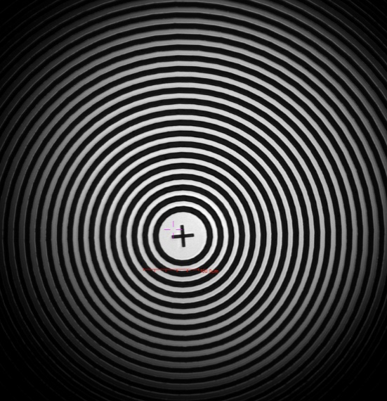
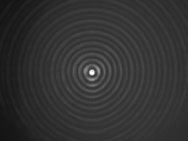
To finish up, here is a microphotograph of the central part of an Axicon grating with 50 lp/mm made by ebeam lithography by Arizona Optical Metrology and the resulting intensity pattern perpendicular to the Bessel beam propagation axis. For scale the FWHM of the core is about 10 µm in diameter.

Further references:

[4] van Heel, A.C.S., “High Precision Measurements with Simple Equipment”, JOSA, 40, 809 (1950).

[5] McLeod, J. H., “The Axicon: A New Type of Optical Element”, JOSA, 44, 592-7 (1954).

[6] Durnin, J., “Exact solutions for nondiffracting beams. I. The scalar theory”, JOSA-A, 4, 651-4 (1987).

[7] Turunen, J., Vasara, A. and Friberg, A., “Holographic generation of diffraction-free beams”, Appl. Opts., 27, 3959 (1988).

[8] Dong, M and Pu, J., “On-axis irradiance distribution of axicons illuminated by a spherical wave”, Optics & Laser Tech., 39, 1258 (2007).