INTRODUCTION
On-machine metrology is particularly important for diamond turning and grinding as it is difficult to remount and align a part if it does not meet off-line inspection criteria. There is also the issue of tool wear; a process that started well may fail part way through the cut, and if tool replacement is needed, it is vital to know that before removing the part. A means of rapid, noncontact, in situ profiling and roughness measurement could improve the productivity of diamond tool machining.
Recently we first showed that diamond turning machines are sufficiently isolated that steady fringes can be obtained by simply setting a Point Source Microscope [1,2] equipped with an interferometric Mirau objective on the cross slide of a machine. Further, we demonstrated that the machine can be precisely driven to get temporally shifted fringes so that common algorithms can be used to obtain area based surface roughness measurements. This led to the question of whether essentially the same hardware could be used to rapidly profile diamond turned parts. We show via simulation that the answer is yes and that the approach can be implemented rather simply.
We first describe the PSM and its configuration as a Microfinish Topographer (MFT) by using interferometric data reduction software. Then we describe how this hardware is changed into a profiler by changing the light source and camera. Finally, we show how this hardware that we call a Non-Contact Profiler [3] (NCP) is used on a diamond turning machine to profile turned or ground parts in situ.
MICROROUGHNESS TOPOGRAPHER (MFT)
The Point Source Microscope [1] has been described previously while the MicroFinish Topographer [2] (MFT) is the same hardware where the LED illumination channel is used as the light source and a Mirau interference objective replaces the standard infinite conjugate objective as shown in Fig. 1.
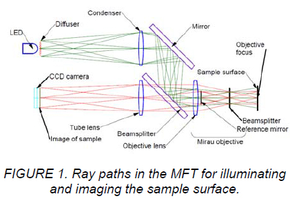
The red LED source has sufficient coherence to obtain interference fringes within about ±8 μm of the reflection from the reference mirror in a 10x Mirau objective. This is more than enough coherence to get surface roughness data over a 1 x 0.75 mm area with a 10x objective as long as the objective reference mirror is within about 1° of the normal to the surface. Higher magnification objectives have proportionally smaller fields of view but can accommodate greater tilt between surface and reference.
Commercially available software drives a PZT behind the objective to shift the fringes to produce roughness data. Alternatively, machine control based software can step the MFT in ¼ fringe intervals to capture 4 or more interferograms, and reduce the data to provide surface roughness information.
WHITE FRINGE LOCATION
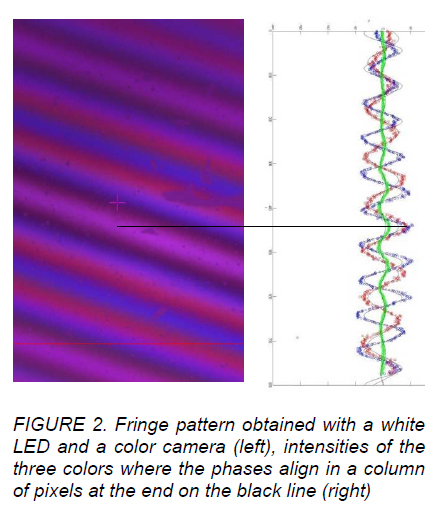
Quite separately from our work on roughness metrology we found that by using a white light LED and a color camera, it is easy to obtain three fringe intensity patterns, one for each color as shown in Fig. 2. When the phases of all three fringe intensity patterns are aligned we get a white or black fringe depending on whether the surface is a dielectric or metal, respectively, indicating that the surface and reference mirror in the objective are precisely conjugate, or the same distance from the beamsplitter. In white light scanning interferometry this is done by looking for a peak in fringe contrast. With the 3 distinct wavelengths in a white LED there are 3 distinct fringe intensity patterns captured by the color camera. On the left of Fig. 2 is the white LED fringe pattern as seen using a 10x Mirau objective and a color camera, while on the right is a plot of the three intensities from one row of the data. The phases of all three sinusoidal intensity patterns from a row of data align at the location of the white fringe as indicated by the black line tying the figures together.
The realization that we could easily recognize the white fringe using the same hardware as the MFT led directly to the idea that the same device used for roughness measurement could be used as an indicator, or sensor, to profile based on the location of the white fringe in the frame of data. We call the MFT used in this way to profile the Non-Contact Profiler (NCP).
INFORMATION IN THE WHITE FRINGE
The information for contouring comes out of the algorithm used to find where the phases align. A sine wave is fit to each of the three intensities in the form I = A*sin(B*x + C). The amplitude A is of no interest while B is proportional to the number of fringes in a frame of data, or the tilt between the reference mirror and the patch of surface observed. For a given frame of fringes, B is also inversely proportional to the wavelength being fit because there will be more fringes for a shorter wavelength. The white fringe is at the value of x (in pixels) where the argument (B*x+C) is equal Nπ/2 for odd integral N. Once B and C are found for each row (or column) of intensity data, the y value (or x value), in pixels, is known for the position where the reference mirror and surface are conjugate, or the same distance from the beamsplitter in absolute terms.
Fig. 3 shows an example of a 2 μinch (50 nm) rms surface from a GAR surface roughness standard artifact [4] with the x,y locations of the center of the white fringe indicated with a row of dots. The scale in the Figure was set by the 10x objective; the optical path difference between fringes for the blue wavelength is about 240 nm and in this example there are about 100 pixels between fringes. Once the fitting is done to find the white fringe, and assuming there are no big jumps from row to row of data, the center of the fringe can be found with a simple algorithm that takes less than 1 ms per row. This means surfaces can be profiled with 1 μm spatial resolution at a rate of 1 mm/sec and proportionally faster at lower spatial resolutions and with height resolutions of a few nm rms.
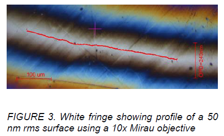
One mode of using the NCP is as an optical micrometer. For example, in Fig. 3 if one wanted to know how far to move the NCP in z to bring the center of the white fringe to the cross, the column of data containing the cross would be fit to find B and C. The C coefficient tells how far to move in nm scaled by the fringe spacing B in pixels per nm.
This mode could be used to find spindle growth by laterally positioning the cross at the vertex of a part and then moving in z to set the white fringe on the vertex. After running the spindle for a time, the movement of the white fringe from the cross gives the spindle growth. Similarly, in the indicator mode, parts could be squared with the face plate.
The usefulness of this mode is that the height or angle of a particular feature in the field of view can be compared to another to a few nm rms or a few seconds of arc for nm or second differences. The sensitivity is proportionally less the greater the difference in feature height or angle unless the diamond turning machine is used to re-position the NCP. If the NCP is repositioned to have just a few fringes in the field of view, the sensitivity is again in the few nm or second regime. Said in another way, the NCP has high sensitivity when used in a null detector mode but features of interest can be selected on a μm scale spatially.
USING THE NCP AS A PROFILER
Using the NCP as a profiler on a diamond turning machine for near flat surfaces means mounting the NCP on the x slide with set and forget adjustments to center the field of view on the spindle axis and a few minutes of arc off normal so there are a few near vertical fringes across the detector. As long as the angle between reference mirror and surface is no more than about 1° for a 10x objective, the white fringe can be kept in its initial position as the x axis is scanned by using the value of C as a feedback signal to the z axis. A safer and more practical mode would be to run the theoretical part curve and record C as a function of the x axis position to create a contour error map.
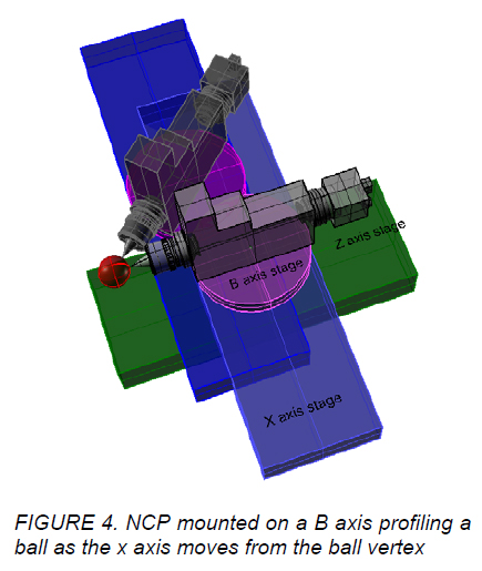
For parts with a steep enough radius to have normals greater than 1° when using a 10x objective, the NCP must be mounted on a B axis rotary table and the B axis used to keep the NCP near normal to the surface as it is scanned in x and z as illustrated in Fig. 4. Again, the most practical method of contouring is to run the part contour path and watch for changes in the white fringe location as the indication of errors in the part.
The distance between the objective focus with the white fringe in the middle of the display and the B axis is the “tool radius” used in calculating the measurement profile. To go from cutting the part to measuring is a matter of changing from the “tool radius” to the “measurement radius” where the measurement radius is pre-calibrated and stored in the machine control software as a new “tool radius”. Clearly, errors in the measurement of the tool radius will lead to errors in the measured contour. However, calibrating the tool radius for measurement purposes is easily done by contouring a good grade steel ball.
Radial errors in the B axis will contribute directly to errors in the measurement of the part contour. However, the oil hydrostatic B axis bearing can be compensated to under 20 nm. Errors in all three angular degrees of freedom in the B axis rotation and axial translation of the B axis make only second order contributions to measurement errors.
Although we have not yet profiled a part on a diamond turning machine, we have simulated real fringe data by thermally changing the optical path between a diamond turned part and the objective reference mirror and shown that the white fringe center can be tracked at 30 frames per second. We have also shown that fringe centers within each frame of data can be found at least as fast as 1 msecond per pixel row or column of data in the frame. This translates to a spatial resolution of 1 μm on the surface using a 10x Mirau objective.
FUTURE WORK
Clearly, our next move is to mount the NCP on a machine and profile a known part. We hope to do this in the next couple of months to obtain data showing in situ profiling performance. In addition, we want to profile a non-rotationally symmetric part. If, using a 10x objective, the normal in the y direction is less than 1°, we can do this profiling with the setup just as described including profiling while the part is rotating on the spindle at low rpm.
Further, surface roughness measurements can be made at any point in the process of profiling by moving in steps normal to the surface. Roughness data can be obtained at angles as great as 1° for a 10x objective as well since the diamond turning machine is well isolated and there is little danger of fringe print through. If the normals are greater than 1° we can go to higher power objectives to get up to 5° off normal with a 50x objective and smaller field of view.
For still greater angles we will have to add an A axis of rotation and use the white fringe position from both row and column data to produce profiles in both the radial and tangential directions. In this case the initial tilt of the NCP to the surface under test would be set to produce fringes at roughly 45° to the machine coordinate system. Further, the profiling could be done on a spiral basis to give areal coverage of non-symmetric and free-form parts.
CONCLUSIONS
We have described a simple method of performing in situ, non-contact profiling of diamond turned parts using a well proven sensor head with a pseudo-white light source and a color camera instead of the normally used red LED and monochrome camera. The color source and camera provide a means of unambiguously isolating the white, or black, fringe that shows precise conjugation of the reference with the surface under test. This permits making profile measurements with a precision of a few nm rms and a spatial resolution of a few μm while taking data at a contouring speed of about 10 mm/second.
For surfaces that depart from plane by 1° or less, all that is required for profiling is a PSM with a Mirau objective, a white light LED source and fairly simple algorithms. This same mode of operation works for angles up to 5° by using a 50x objective although proportionally smaller fields of view are seen.
For symmetric surfaces with larger slopes, the sensor head must be mounted on a B axis to keep the number of fringes from becoming to great to resolve. For steep non-symmetric surfaces, an A axis must also be added. In addition to this profiling capability, there is the
simultaneous ability to measure surface roughness by stopping the scan and obtaining 4 or more interferograms at the desired location. No additional alignment is necessary because the NCP is already near normal to the surface, and the machine motion control can do the phase stepping.
REFERENCES
- Parks, R. E., “Versatile Autostigmatic Microscope”, Proceedings of SPIE Vol. 6289, 62890J, (2006).
- Parks, R. E., “Micro-Finish Topographer: surface finish metrology for large and small optics”, Proceedings of SPIE Vol. 8126, 8126- 11, (2011).
- Non-Contact Profiler, patent pending
- garelectroforming.com/s- 22_Microfinish_Comparator.htm