I was never satisfied with my explanation of lens centering, so this Chapter is another try. Start with a diagram that is familiar to anyone who has some familiarity with optics, the diagram that explains first order image formation as in Fig. 1.
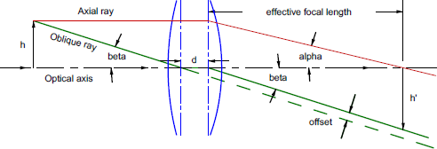
Fig. 1 A generic optical system with the two rays that define an axial and an oblique ray.
Keeping the discussion general I use Warren Smith’s labeling of the rays as “axial” if the rays are parallel to the system optical axis without specifying a height. An “oblique” ray is any ray that is not parallel to the system optical axis.
In the paraxial case, an axial ray is parallel to the optical axis until it arrives at the second principal plane where it abruptly changes direction and crosses the optical axis at the focal plane. An oblique ray goes directly to the first principal plane where it bends parallel to the optical axis and proceeds to the second principal plane. There it bends again so the ray is parallel but not coaxial with the incident ray. The dotted green line shows the offset of the ray due to the ray being incident at an angle, β, to the optical axis, the line joining the two centers of curvature in the case of a single lens element. An oblique ray will always suffer an offset equal to β·d.
The first order, or paraxial, relations of interest are
𝛼 = ℎ
𝑒𝑓𝑓𝑒𝑐𝑡𝑖𝑣𝑒 𝑓𝑜𝑐𝑎𝑙 𝑙𝑒𝑛𝑙𝑙𝑡ℎ
= ℎ/𝑒𝑓𝑙 (1
and
𝑜𝑓𝑓𝑠𝑒𝑡 = 𝛽 ∙ 𝑑 (2
where, d, is the distance between the principal planes. A ray incident along the optical axis propagates through the lens system undeviated.
To see how this relates to lens centering, consider Fig. 2 where the incident axial ray propagates coaxial with our reference axis. To the right, we have set up a position sensitive detector centered on the reference axis prior to inserting the lens. This means that when the lens is inserted as pictured, optical axis is decentered by a distance, h, and the axial ray is deviated by the angle, α.

Fig. 2 Axial ray incident along the reference axis so the lens system is decentered by h
If the lens were rotated about the axial ray and reference axis, a sensor in the focal plane would see the image rotate in a circle with a diameter of 2h. Moving the lens up until the second nodal point was on the reference axis would make the ray continue to propagate coaxially with the reference axis and eliminate the motion.
The picture gets more complicated if we assume that the oblique ray is our reference axis as in Fig. 3.
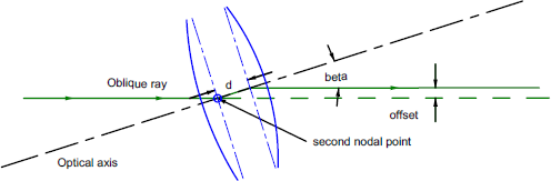
Fig. 3 Using an oblique ray as the reference axis
This situation illustrates the case where we have a tilted lens or optical system. Our sensor is set up centered on the green dotted line, which is the extension of the incident ray. The tilt of the lens displaces the ray yet the incident and exiting rays are precisely parallel. The offset, although generally small, cannot be eliminated unless β = 0, in which case we have an axial ray
The only way to eliminate both the angularly deviated ray in the case of decenter and the offset in the case of tilt is to align the lens’ optical axis with the reference axis along which the ray is incident. This requires adjustments in both tilt and decenter. In some centering situations this is impossible given the mechanical constraints of the cell or tolerances on the lens. Is there a best compromise between tilt and decenter in this situation?
Fig. 4 suggests the solution. Assume a centroiding sensor is centered on the incident ray that we use as a reference axis as in 4a. Then a tilted lens is inserted in the path where just the principal planes and nodal points are shown for clarity in 4b-d. Once the lens is in the ray path, the oblique ray is parallel with the lens’ optical axis between the principal planes making it an axial ray in that space. When the incident ray is directed at the first nodal point as in Fig. 4b, the ray exits at the height of the second nodal point and
parallel to the incident ray.
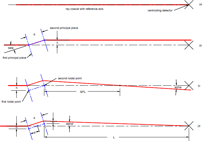
Fig. 4 Effect of incident oblique ray height on the exiting ray height and angle
If the ray is incident at the height of the second nodal point as in 4c, that is, at a distance h = β·d above the first nodal point, the ray bends at the second principal plane to pass though the reference axis at the focal point. If the centroiding detector is anywhere but at the focal point the ray is not centered on the detector.
In Fig. 4d, if the ray is incident at any height between these two cases, that is, 0 < h’ < h = β·d, the ray exits at some height less than the total offset β·d and crosses the lens optical axis at some point, L, beyond the focal plane at an angle α’ less than β·d /EFL. Note the ray crosses the lens’ optical axis between the two principal planes.
In Fig. 4d, the offset of the ray going through the lens is still h = β·d because all we have done is decenter the lens with respect to the incident ray. However, the ray angle α’ of the ray exiting the lens is decreased in angle by the same ratio as h’/h = d’/d. The reduced angle means the ray is centered on the detector when L = α’/h. If the detector is farther from the lens than the EFL and exiting ray is centered on the detector, we know that when the ray enters the lens at a height between 0 and h, the lens’ optical axis crosses our reference axis between the nodal points.
There are several consequences of this situation: in general, the tilt of single lenses is small, typically 1
milliradian or less, and for typical lenses the distance between principal planes is a few mm. This means that the location of the principal planes can be measured to a few µm and the angle of the exiting ray kept to a few arc seconds. Also, because the ray and lens’ optical axis cross between the principal planes, the centers of curvature will not lie on the reference axis. If the single lens is mounted in a cell that constrains an alignment degree of freedom, the remaining degree of freedom is used to keep the principal planes centered on the reference axis by seeing that the exiting ray is centered on the detector.
This method of alignment works in a strictly x-y coordinate system and gives immediate feedback about the ray position on the detector without having to move any part of the measurement apparatus. All that is needed is a device to make a Bessel beam that serves as the reference axis and a position sensitive detector to centroid on the Bessel beam.
Another consequence of this method is that it applies to whole lens assemblies because an assembly will also have principal planes. Moving the centroiding sensor several focal lengths from the lens lets you center the lens on the reference axis between the principal planes. This is handy if the lens cell defines the tilt of the lens. You now know the precise center of the field on any camera you attach to the lens.
In a future Chapter, we will discuss further consequences of this centering method and what can be learned about the quality of lens assemblies from how well they are centered.