ABSTRACT
In many lens assemblies, mounting constraints prevent independent adjustment of tilt and decenter making perfect alignment of individual elements impossible. This work models a plano-convex lens to compare several centering methods under partial constraint, including mechanical edge runout, image runout, center of curvature centration, and transmitted Bessel beam deviation. Although based on a single element, the results provide insight into alignment strategies for more complex systems. Of the methods evaluated, Bessel beam centering aligns the lens optical axis to a reference axis as well as or better than the more traditional methods. It is also the simplest method and least expensive to implement, making it a practical solution for aligning partially constrained lenses.
- INTRODUCTION
In many lens assemblies, mounting features constrain the independence of tilt and decenter for individual elements, making it impossible to perfectly align an element’s optical axis to a reference axis. This raises a practical question: how do we best center a partially constrained lens to minimize system performance degradation?
To answer this, we model a plano-convex lens to compare centering methods while the element is constrained by its seat. Evaluating alternative centering criteria provides insight into how alignment choices influence the location of the optical axis relative to the assembly’s reference axis, and by implication, the axes of other lenses in the assembly.
The centering methods examined include mechanical edge runout indication, center of curvature (CoC) runout, image runout observed during rotation on a precision bearing, and deviation of a transmitted Bessel beam. We show that mechanical runout, or edge thickness difference, produces the same geometrical alignment of lens optical axis as centering CoCs, and that centering by image motion is similar to centering with a Bessel beam because both methods force the nodal points on or near the reference axis.
To assess centering performance, we consider the relationship of the lens optical axis to a reference axis and the deviation of a ray propagated into the lens along that reference axis. Among the methods investigated, Bessel beam centering produces the best alignment of the optical axis to the reference axis. In addition, this method is the simplest to implement and requires the least specialized hardware. Because the hardware remains stationary throughout the process, this approach offers a clear path toward automated lens centration.
We begin by describing the parameters of the example plano-convex lens we use to compare the various methods of alignment so that we have a common measurand for comparison of the methods of centering. Then we describe the two common cases of misalignment, one in tilt and one in decenter that are considered in each method of alignment. With this background, we look at centering by mechanical means, look at the runout of centers of curvature and image motion as a lens is rotated about an axis, and centered using a Bessel beam as the reference axis. Finally, these four methods of centering are compared in terms of the relationship of the lens optical axis to the reference axis and the deviation of a beam propagated through the lens along the reference axis.
- EXAMPLE LENS PARAMETERS USED FOR THIS STUDY
2.1 Basic Lens Parameters
To compare centering methods quantitatively, we use a plano-convex lens with a 100 mm effective focal length (EFL), a 50 mm convex radius, a 4 mm center thickness, and a refractive index of 1.50 as shown in Fig. 1.The first nodal point and “optical center” reside at the first surface. The second nodal point sits at 1.333 mm, and the apparent center of curvature after refraction through the plano surface is at 34.286 mm. Both optical and mechanical CoCs lie on the optical axis.
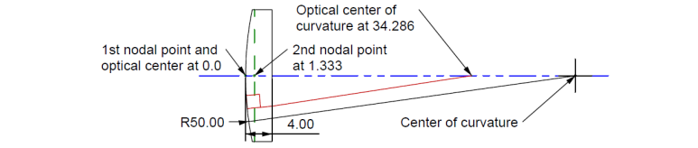
FIG. 1. Parameters of the model plano-convex lens used for the centering calculations.
In a perfectly centered lens, the optical and mechanical axes coincide, making it difficult to show in the Figures, so we use only one axis in this case. For the reference axis, generally the z axis of the global reference system used for lens design ray tracing, we use a dashed line.
2.2 Optical Center of a Lens
The “optical center” of the lens mentioned above is sometimes referred to as the seventh cardinal point of a lens [1], and is a useful datum when discussing centering.
A “nodal ray,” a ray aimed at the first nodal point, see Fig. 2, enters the lens and then emerges from the second nodal point with the same angle as it entered. The internal real ray segment crosses the optical axis at the “optical center.”
For the entry and exit angles to match, the local surface regions intersected by the ray must be parallel, causing the lens to locally act like a plane-parallel plate.
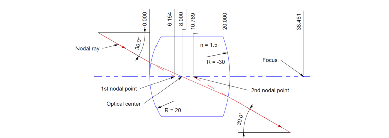
FIG. 2. Example of the “optical center” of a lens as the place where a “nodal ray” crosses the optical axis.
The distance from the first surface vertex to the optical center (t_oc) is given by:
t_oc = t × r₁ / (r₁ − r₂)
where t is the lens center thickness, and the r’s are the radii of the first and second surfaces.
Fig. 2 is based on a similar figure in the reference [1], but I chose to show a specific numerical example so that you can see how the dimensions were derived and why the optical center is a useful concept when discussing centering.
Because this expression is purely geometric and depends solely on surface radii and thickness rather than refractive index, it serves as a constant, unambiguous, single-point datum referenced to the first surface vertex.
For our example plano-convex lens (r₂ = ∞), t_oc = 0, meaning the optical center coincides exactly with the vertex of the convex surface.
- MISALIGNMENT CONDITIONS
We evaluate two explicit initial misalignments: a 1 milliradian tilt and a 0.1 mm decenter as shown in Fig. 3.
The 1 milliradian tilt corresponds to the plano side resting on a seat tilted relative to the reference axis, with the only allowed centering adjustment restricted to sliding along the seat. Another way of thinking of this misalignment condition is that the lens is rotated about its first surface by 1 milliradian.
The 0.1 mm decenter corresponds to a seat offset from the reference axis with the centering adjustment restricted to rotating the lens about its center of curvature, which simultaneously changes tilt and decenter.
Fig. 3 shows these two arbitrary misalignments prior to correction. With this background, we will now look at several methods of centering correction limited by these constraints.
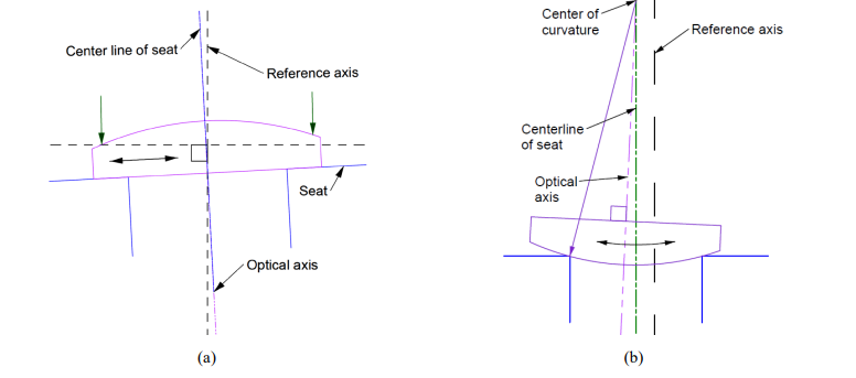
FIG. 3. The two alignment situations considered: (a) where tilt is constrained, and (b) where decenter is constrained by the seat.
- CENTERING CORRECTION UNDER CONSTRAINTS
4.1 Centering Correction by Minimizing Edge Thickness Difference (ETD)
Before optical methods were common, lenses were checked for centration using a dial indicator and a fixture that defined five degrees of freedom. Three small balls constrain lens tilt by supporting one surface, while two larger balls constrain centration along the outer periphery (Fig. 4).
The difference between the maximum and minimum indicator readings after a 180° rotation is the ETD. A lens with wedge shows a height change under the indicator (Fig. 5). The wedge angle relates to ETD by dividing the thickness difference by the lens diameter.
Centering using ETD is also performed by directing a laser beam at an unconstrained lens surface (Fig. 6). If ETD is zero, the reflected beam remains stationary as the lens rotates on a true running cup.
Because the optical axis of a single element is defined by the two centers of curvature, making ETD go to zero is functionally equivalent to aligning the CoCs to a reference axis. Consequently, we treat ETD and optical CoC centering as one in the same.
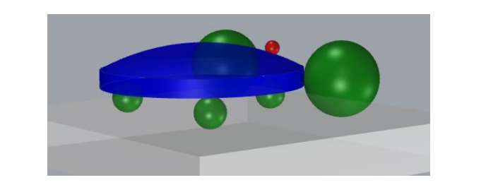
FIG. 4. Five-constraint fixture for measuring ETD with an indicator tip (red ball).
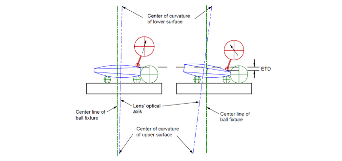
FIG. 5. Lens with wedge being measured for ETD at maximum and minimum thicknesses.
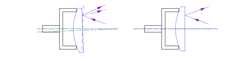
FIG. 6. Lens mounted on a true running cup, misaligned (left), where the dotted line shows the surface rotated by 180 degrees, and aligned (right), where the reflected spot is stationary.
4.2 Quantitative Effects of Centering by ETD and CoCs When the Centering Is Constrained
Centering the tilted lens demands that we slide it (decenter it) along the tilted seat because it is constrained by the seat.
We slide it until the upper surface center of curvature lies on the reference axis, which brings the ETD to zero.
Correcting the decentered lens requires rotating it about its center of curvature until the tilt is eliminated, which zeroes the ETD but leaves the CoC of the lens offset from the reference axis because the seat is decentered from the reference.
Fig. 7 shows the lens after these two corrections are made using a zero ETD.
In the tilted case, Fig. 7a, the initial 1 milliradian tilt displaces the center of curvature by 46 µm from the reference axis because it is 46 mm from the seat. Decentering the lens by 46 µm makes the ETD zero.
If a ray enters the lens along the reference axis it exits 1.33 µm from, and at an angle of 487 µradians relative to the reference axis.
This matches first-order predictions for a 4 mm thick plate tilted by 1 milliradian and a thin prism with 1 milliradian of wedge.
Note, the optical and reference axes intersect at the center of curvature in the case of the tilted seat.
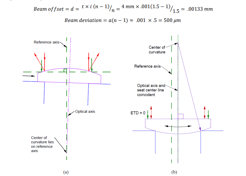
FIG. 7. Tilted lens with misalignment corrected by decentering (a) and decentered lens with misalignment corrected by rotating about its center of curvature (b).
In the corrected decentered case, Fig. 7b, a zero ETD occurs when the plano surface is parallel to the seat.
An incident ray along the reference axis is parallel to the optical axis but displaced by 0.1 mm. The ray exits at a height of 97.33 µm and an angle of 1 milliradian relative to the reference axis, matching expectations for a 97.33 mm back focal length.
The ray travels parallel to the optical axis until the second principal plane, then refracts toward the focal point. In this case, the optical and reference axes remain parallel and there is no way to change this and keep the ETD zero.
Note that our example plano-convex lens lies about midway between extremes of centering.
At one extreme is a ball lens where the CoCs are coincident and it is impossible to misalign the lens by tilting about the CoC. At the other extreme is a lens with two strictly concentric surfaces where again the CoCs are coincident.
In both cases there is no optical axis, and the only misalignment is decentration.
4.3 The Effect of Centering a Constrained Lens by Means of Image Motion
In image-motion centering, the lens is illuminated with a point source or a collimated beam. The focused image is observed through a microscope while the lens rotates about a mechanical reference axis.
If the optical axis is misaligned relative to the rotation axis, the focused spot traces a circular path in synchronism with the rotation.
Consider our plano-convex lens (t = 4 mm, EFL = 100 mm) resting on a seat with a 1 milliradian tilt (Fig. 8a).
If the optical axis intersects the reference axis at the plano surface, the optical axis will be offset by 4 µm at the convex vertex. Because the second nodal point lies at the convex vertex, the nodal point is displaced by 4 µm from the reference axis.
A beam propagating along the reference axis refracts at this surface and focuses 100 mm away, displaced 4 µm from the reference axis. Rotating the lens causes this spot to sweep out an 8 µm diameter circle.
Centering the lens to eliminate this image motion means translating the lens 4 µm laterally to align the nodal point with the reference axis.
This shift moves the CoC of the convex surface to 50 µm from the reference axis, combining the initial 46 µm tilt offset with the 4 µm lateral translation.
Once corrected, the image remains stationary during rotation, and the optical axis intersects the reference axis at the convex surface vertex.
A ray incident along the reference axis emerges from the convex surface 1.33 µm from the reference axis and at an angle of 13.3 µradians relative to it.
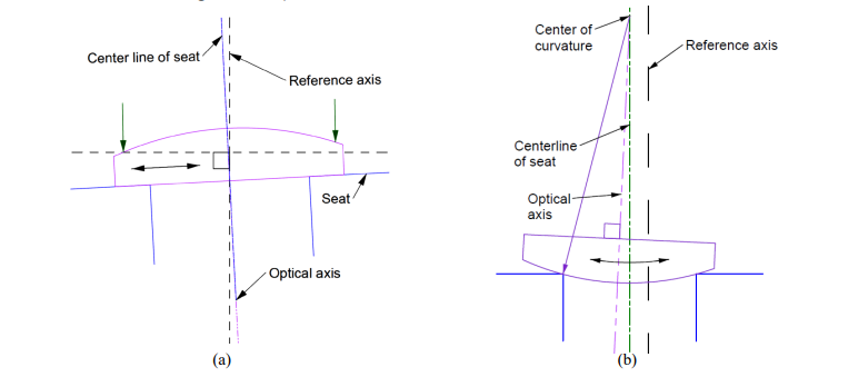
FIG. 8. The tilted seat (a) and the decentered seat (b) prior to correction by viewing image motion.
For the decentered seat (Fig. 8b), the CoC remains fixed at 0.1 mm from the reference axis regardless of the lens tilt.
Sliding the lens across the seat until the optical axis lies within 2.77 µm of the reference axis centers the image spot on the rotation axis, eliminating image motion.
At this position, the optical axis forms an angle of −0.1176° relative to the reference axis. A ray incident along the reference axis emerges 2.67 µm from the reference axis and at an angle of −27.6 µradians relative to it.
The optical and reference axes intersect 1.343 mm behind the convex vertex, about 10 µm beyond the second nodal point.
4.4 Centering Using a Bessel Beam
Ever since reading papers describing Bessel beam propagation as an ABCD ray [2], [3], we have been experimenting with the use of Bessel beams for optical centering.
Rather than illuminating an Axicon or grating of concentric, equally spaced rings with a collimated wavefront, we have been using a spherical wavefront to produce a Bessel beam that has an extended length rather than a finite one.
In this case, the core of the beam does not remain strictly the same diameter but slowly increases with propagation distance.
As a practical matter, if the Bessel beam lateral position is measured at about 10 times the lens element focal length, the increase in the diameter of the core remains small and well within the typical field of view of a 10x microscope objective.
For our example, we assume our detector is located 1 m from our 100 mm EFL lens. Prior to inserting our lens in the Bessel beam, our detector, in this case a Point Source Microscope (PSM), is centered on the Bessel beam.
As in the previous cases of centering, we slide the lens on the tilted seat until the Bessel beam is again centered on the PSM.
If the lens were inserted so that center of the plano surface was centered on the Bessel beam used as our reference axis, the beam would be displaced 28.0 µm at the PSM.
This is just the situation you would have in a lens design program if you tilted the plano-convex lens about the plano surface, the point of rotation would be about the global reference axis and the vertex of the plano surface.
Sliding the lens 2.80 µm centers the beam on the PSM.
Because the tilted seat means the CoC is already 46 µm from the reference axis when the lens is centered on the plano surface, the CoC is now 48.8 µm from the reference axis.
Further, the ray enters at 2.80 µm from the optical axis and exits at −1.33 µm and at an angle of 1.3 µradians relative to the reference axis.
This means that the optical and reference axes intersect at 1.20 mm from the convex surface, a location between the nodal points.
In the case of the decentered seat, we can model the situation as if the lens is initially decentered by 0.1 mm, so the gut ray is incident on the lens 0.1 mm from the optical axis.
This displaces the ray by 1003 µm at the PSM 1 m away.
By sliding the lens in its seat to bring the Bessel beam back to the center of the PSM, it takes a rotation of −0.1149° about the CoC.
The ray now exits the lens at 2.67 µm and an angle of 2.7 µradians relative to the reference axis.
The optical and reference axes intersect at 0.133 mm, again between the nodal points and close to the optical center.
It is beyond the scope of this paper, but it can be shown that if the Bessel beam lateral position is centered at any axial distance beyond the lens focus, the optical and reference axes intersect between the principal planes [2].
In the case of our model lens with a maximum tilt of 1 milliradian, this is an area 1.33 mm long by 1.33 µm wide, a tight localization for a simple method of centering.
4.4.1 Sensitivity and Quick Test of Centering with a Bessel Beam
For our example, since the detector is 10 times the EFL from the lens and the sensitivity of the PSM to centroid location is < 1 µm with a 10x objective, this means that using a Bessel beam there is centering sensitivity in the nm range.
Coupled with this sensitivity and going back to the 5-degree-of-freedom (DOF) constraint fixture, there is an easy and sensitive test for a combination of lens diameter and centration.
If the lens is not the correct diameter to match the large ball constraint, then the Bessel beam will be deviated to a fixed location from the centered position in a plane that bisects the ball locations independent of the rotation of the lens in the fixture.
With the PSM at 10 times the focal length, a 1 µm difference in diameter will displace the Bessel beam by 10 µm at the PSM.
If the lens is the correct diameter to match the fixture but has a wedge of 1 second of arc, the Bessel beam will be deviated by 2.5 µm for our model 100 mm EFL lens and the PSM at 1 m from the lens in the direction of the wedge.
Rotating the lens 180° will deviate the beam the same amount in the opposite direction for a total shift of 5 µm.
While the deviation is directly related to the lens EFL, both the diameter and wedge are checked quickly to high precision in a simple test where the lens is inserted in the 5-DOF fixture and a deviation noted, then rotated 180° and the deviation noted again.
This is the same as the ETD test for centration but now you get twice the information at greater sensitivity.
- COMPARISON OF CENTERING METHODS
We have looked at centering using ETD and shown that this yields the same results in terms of optical axis location as centering by CoCs, so the results of these two methods are shown as one. We also looked at centering by minimizing image motion as the lens rotates about its axis and centering using a Bessel beam that simulates a single ABCD ray. Table 1 summarizes these results. For each method, we have a case each for the tilted seat and the decentered seat relative to the reference axis. The axis intersections are measured from the optical center in mm.
The three basic methods of centering are color highlighted. In the first row of Measurement, we note the magnitude of the centering correction required given the constraints we imposed. For the tilted seats we can decenter with units of µm, and for the decentered seat we give the angle of rotation about the lower surface CoC in µradians.
The NA listed for the ETD method for the decentered seat means that if we are holding one center of curvature to the reference axis to make the ETD or CoC zero, there is nothing more we can do to improve centering. The optical axis in the case of our plano-convex lens will be parallel to the reference axis. If both surfaces are powered so it is a bi-convex lens, the two axes will cross closer to the physical center of the lens the more equal the power of the surfaces. The plano-convex example is a worst case for ETD or CoC centering.
The next two lines show the ray angles and heights relative to the reference axis of the emergent ray after centering correction when an incident ray is coaxial with the reference axis. While the ray heights are the same for all methods, the emergent ray angles differ significantly, with the ETD method being the worst.
FIG. 9. Table 1. Comparison of methods of centering.
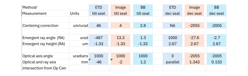
The last two lines show the angle of the optical axis after centering correction and the place along the optic axis that the ray incident along the reference axis intersects the optical axis relative to the optical center. The angle is the same for all tilted seat cases because that is our constraint. For the decentered seat, there is substantial difference between the ETD method and the other two. In several cases the values are 10 times larger for image motion than for BB centering. This is because we are making our correction based on a measurement made 10 times as far from the lens.
We have already noted that ETD and CoC centering lead to the same geometric results. In the worst case, the optical and reference axes remain parallel but displaced after centering, as in our plano-convex example. With a second powered surface, one center of curvature will lie on the reference axis while the other does not given our constraint.
Similarly, image motion and Bessel beam centering produce much the same result because they both force the nodal points close to the reference axis. This, in turn, means that the CoCs lie on either side of the reference axis when the lens is centered under our constraints. The main difference in the techniques is that the Bessel beam is detected farther from the lens than for image motion, which makes the Bessel beam method more sensitive by the ratio of Bessel beam measurement distance to the lens EFL.
Note that the values after correction are smaller in all cases for the Bessel beam method where allowed corrections were made given the constraints. Also, the ray incident along the reference axis intersects the optical axis between the principal planes only in the case of the Bessel beam method. This means that our example lens is centered laterally so that the ray is within ±0.7 µm of either nodal point for either tilt or decenter initial misalignment.
- CONCLUSION
We have discussed and compared three different methods of centering single lens where one of the degrees of alignment freedom is constrained. The newer method using a Bessel beam appears better than the traditional methods. Does this mean that the centering we have done all these years was wrong? Not at all. It is that we now have a new tool in the Bessel beam that allows us to do better than in the past.
It is like the invention of phase shifting interferometry. We could not do daily interferometric testing if the HeNe laser had not been invented in the 1960s. The Bessel beam was not available as a tool until it was theoretically realized that it propagated as an ABCD ray [3] some 9 years after the idea of a Bessel beam was formally introduced in the literature [4]. It took another 27 years to recognize that the ABCD ray propagation property of the Bessel beam might have a practical application in the alignment of optical elements [5].
It is our hope that these insights will promote more discussion about alignment methodology to verify some of the conclusions in this study. Assuming they are correct, and we believe they are, the use of a Bessel beam for alignment should have an impact on the tolerancing for centering and the methods of lens mounting where there are constraints.
Finally, because it is not necessary to rotate a lens when using a Bessel beam for centering, it means that the route to automated alignment is much easier to implement. Also, better alignment is possible because of the greater sensitivity to alignment errors. This leads to better optical system performance.
REFERENCES
[1] R. Kingslake and R. B. Johnson, Lens Design Fundamentals, 2nd Ed., SPIE Press, (2010), pp. 75–77.
[2] https://medium.com/@reparks_11319/chapter-26-single-lens-centering-435e47278155
[3] Santarsiero, M., “Propagation of Generalized Bessel-Gauss Beams through ABCD Optical Systems,” Optics Communications, 132 (1996), 1–7.
[4] J. Durnin, “Exact Solutions for Nondiffracting Beams. I. The Scalar Theory,” JOSA-A, 4(4), 1987.
[5] Parks, R. E. and Kim, D., “Physical Ray Tracing with Bessel Beams.” In Proc. of ASPE Spring Topical Meeting, Tucson, AZ. 2023.