Authors: Zhaowei Chena, Ryan Luua, Robert E. Parksb, Surya Prakash Gurunarayananc, and Daewook Kima,*
- a James C. Wyant College of Optical Sciences, University of Arizona, 1630 E. University Blvd, Tucson, AZ 85721, USA
- b Optical Perspectives Group, LLC, 7011 E. Calle Tolosa, Tucson, AZ 85750, USA
- c ASML US, LP, 77 Danbury Rd, Wilton, CT 06897, USA
- *Send correspondence to Daewook Kim (E-mail: optjcs@gmail.com) or Zhaowei Chen (E-mail: chenz11@arizona.edu)
ABSTRACT
We present a deep-learning-based phase-retrieval framework that uses Bessel-beam illumination to extend the recoverable aberration range in wavefront sensing. By exploiting the large effective numerical aperture and extended depth of focus of Bessel beams, the proposed method increases the range of measurable aberrations compared with conventional Gaussian-beam-based approaches while preserving high reconstruction accuracy. A linear grating is used to generate off-axis Bessel-beam orders, providing additional spatial information that enables single-shot phase retrieval from one measured irradiance image. To address the nonlinear inverse mapping from defocused Bessel-beam irradiance patterns to wavefront aberration coefficients, we develop a three-stage hybrid reconstruction pipeline. A convolutional neural network first estimates 25 Zernike coefficients, from Z4 to Z28, providing a coarse initial reconstruction. A physics-informed neural network then refines the estimate by enforcing consistency with a fully differentiable Fresnel propagation model. Finally, gradient-based iterative optimization further improves the solution by minimizing a composite loss that compares predicted and measured intensities in the spatial, spatial-frequency, and gradient domains. In noise-free simulations over 100 test cases with wavefronts spanning up to 7.3λ peak-to-valley, the full pipeline achieved a wavefront reconstruction error of approximately 1.4 nm RMS at λ = 632 nm. These results show that structured Bessel-beam illumination, combined with hybrid data-driven and physics-based inference, enables fast, robust, and accurate wavefront reconstruction. The approach also supports characterization of test optics over a broad range of effective focal lengths without optical reconfiguration, offering a flexible wavefront-sensing strategy for imaging and metrology applications.
Keywords: wavefront sensing, Bessel beam, phase retrieval, deep-learning, machine learning
1. INTRODUCTION
Phase retrieval (PR)1 is a computational method for recovering wavefront phase from irradiance measurements. Most conventional PR systems use Gaussian-beam illumination because it is readily available and well behaved. However, Gaussian-beam-based PR is limited by two major factors. First, the inverse problem is highly nonlinear, and optimization methods such as gradient descent2,3 become less reliable when the initial phase estimate is far from the true solution. This sensitivity restricts the recoverable dynamic range. Second, the retrievable phase information is constrained by the measured irradiance distribution itself. Conventional PR typically requires measurements near the focal plane, where spatial-frequency information is best preserved.4 As the measurement plane moves away from focus, this information is progressively degraded by the broadened point spread function (PSF). As a result, conventional PR is limited by both the optimization process and the physical information content of the measured signal.
To address these limitations, we propose a deep-learning-based phase-retrieval framework using Bessel-beam illumination.5 A key advantage of a Bessel beam is its ability to maintain a concentrated central peak over an extended propagation distance, which can reach the meter scale.6 By leveraging this extended depth of focus, phase information can be retrieved at planes far from the system focus.7 The method can also recover non-converging wavefronts, thereby expanding the flexibility of practical optical system design.
From a machine-learning perspective, the phase-retrieval task considered here can be formulated as an ill-posed inverse regression problem, in which distinct aberration states may generate irradiance patterns with similar global structure, especially under large wavefront errors. Within this framework, the neural network functions not merely as a fast predictor, but as an amortized inverse model that learns a data-driven prior over physically plausible aberrations from simulated examples.8,9 This prior guides the reconstruction toward a favorable region of the solution space. A physics-informed refinement step then improves the estimate by re-rendering the predicted wavefront through the optical forward model and minimizing the residual against the measured irradiance data. The result is further refined by classical iterative optimization to approach physics-limited accuracy.
Because the measurements consist of structured Bessel-beam irradiance images, a convolutional neural network (CNN) is a natural choice for the inverse model. The CNN can efficiently learn hierarchical spatial features, including ring morphology, radial spacing, and irradiance redistribution, that are difficult to represent analytically in closed form. In this way, the proposed framework combines the broad initialization capability of data-driven inference with the final precision of iterative optimization.
By addressing these two fundamental limitations of PR, the proposed method reconstructs phase information from a single irradiance image containing three PSF orders generated by a linear grating. The irradiance image is fed into a hybrid physics-informed phase-retrieval pipeline to retrieve the phase map at the designated observation plane. This method represents a general framework that can be adapted to multiple applications, although its dynamic range and accuracy depend on the specific system configuration. In this work, we present a case in which a deformable mirror (DM) is used as the target phase plane, and three Bessel-beam orders are generated using a 4 lp/mm linear grating. The optical layout and experimental setup are shown in Fig. 1.
2. PROPERTIES OF THE BESSEL BEAM
The concept of the Bessel beam originates from Durnin’s seminal work on nondiffracting beams.5 Owing to their distinctive properties, including diffraction-resistant propagation and extended depth of field, Bessel beams have been widely used in imaging,7,10 free-space optical communications11 and optical alignment.12 As shown in Fig. 2, the transverse irradiance profile of a Bessel beam consists of a series of concentric rings, and its cross section is described by the squared magnitude of a Bessel function. In theory, an ideal Bessel beam can propagate indefinitely without changing its transverse profile. In practice, however, the nondiffracting propagation length is finite. Even so, in our experiment, the quasi-Bessel beam profile was clearly maintained over a propagation distance of more than 2 m.
Our phase-retrieval strategy is motivated by this extended propagation property. Conventional Gaussian-beam-based PR relies on recording irradiance distributions near the focal plane, where phase-dependent spatial features are preserved most strongly. In contrast, as illustrated in Fig. 3, the Bessel beam generated by the axicon grating maintains its characteristic structure over a much longer propagation distance. Therefore, even at planes far from the nominal focus, the measured PSF can retain distinguishable aberration-dependent features that encode phase information.
Denoting the Bessel wavefront before the phase plane as U1, the field at the observation plane, U2, can be expressed as:

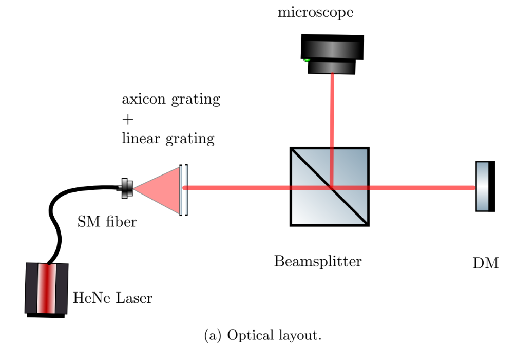
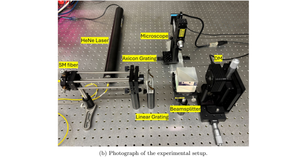
Figure 1: Optical layout and experimental setup. (a) Schematic of the optical system. The single-mode (SM) fiber source is positioned 242.7 mm upstream of the axicon grating, which has a cone angle of 0.0458 rad. The beam then propagates through the linear grating and reaches a beam splitter, where the optical path is divided into two arms. One arm is directed to the DM, with a grating-to-DM distance of 298 mm, and the other arm is directed to the observation microscope. The propagation distance from the DM to the observation plane is 457 mm. (b) Labeled photograph of the corresponding experimental setup.
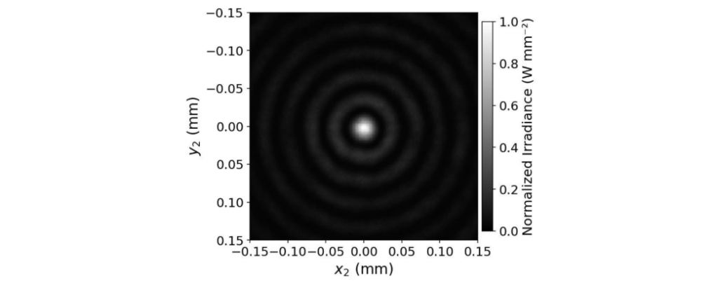
Figure 2: Experimentally generated Bessel beam using an axicon grating, with a central core size of approximately 30 µm.

Figure 3: Schematic drawing of Bessel-beam generation and propagation.
This expression shows that the observation-plane field is determined by the Fourier transform of the phase-modulated field after the lens, convolved with the Fourier transform of the aberration distribution at the lens plane. It also indicates that the information encoded in the measured irradiance pattern is fundamentally constrained by the PSF at the observation plane. Because the system uses coherent illumination, this convolution is not directly reversible from irradiance alone. PR therefore requires an inverse reconstruction strategy, typically involving iterative optimization.
2.1 Bessel beam vs. Gaussian beam
Figure 4 compares the Bessel beam and Gaussian beam under the same optical configuration, with 1 wave of astigmatism introduced at the lens plane. For demonstration, a collimated input wave and a positive lens with an effective focal length (EFL) of 500 mm were used. As the defocus distance increases, the Gaussian-beam PSF expands across the sensor plane, causing the low-order aberration features to degrade. In contrast, the Bessel-beam PSF preserves aberration-dependent structures that remain visually distinguishable over a longer propagation range. This comparison supports the use of Bessel-beam illumination as an effective phase encoder for PR over an extended axial range. The remaining task is to invert the encoding described by Eq. 1: given a single measured irradiance pattern, recover the Zernike coefficients that produced it.
After establishing the physical differences between the phase-modulated Bessel- and Gaussian-beam PSFs, we next evaluate how effectively phase can be recovered under each illumination condition. The same optical configuration was used, consisting of a lens with an EFL of 500 mm and a 4 lp/mm linear grating to generate three distinct PSF orders. The initial-guess RMSE refers to the difference between the starting phase estimate and the reference phase.
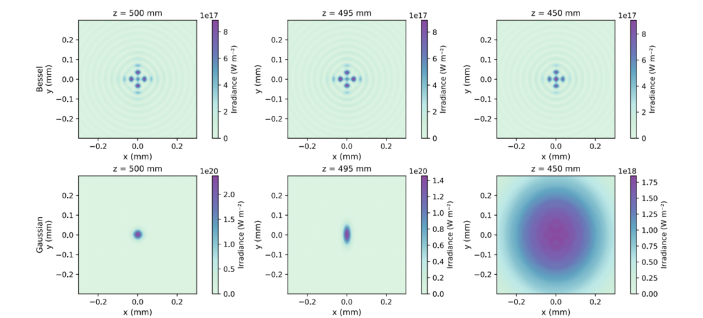
Figure 4: Defocused PSFs of the Bessel beam and Gaussian beam under the same astigmatic aberration.
As shown in Fig. 5, Bessel-beam-based PR tolerates an initial-guess RMSE of approximately 0.65λ, whereas Gaussian-beam-based PR succeeds only up to approximately 0.45λ. This result indicates that Bessel-beam illumination provides a larger capture range for PR.
We also compare the sensitivity of the two illumination conditions to axial misalignment. Here, the z misalignment represents an error in the assumed observation-plane distance. Because the axial position is a sensitive parameter and is difficult to calibrate precisely in practice, tolerance to z misalignment is important for experimental PR. The comparison shows that the Bessel beam is more tolerant of z misalignment than the Gaussian beam, providing another advantage for Bessel-beam-based PR.
3. PHASE RETRIEVAL METHOD
Having shown that the Bessel beam can serve as an effective physical encoder of phase information, the remaining task is to recover that information from the measured irradiance distribution. This inverse problem is highly nonlinear: different Zernike coefficient vectors can produce irradiance patterns with similar global structure, and the loss surface between predicted and measured intensities contains many local minima. Figure 6 illustrates this difficulty using a two-dimensional slice of the loss landscape along the Z7 (horizontal coma) and Z11 (spherical aberration) axes. Multiple local minima are visible even in this restricted view. In the full 25-dimensional parameter space, the large number of such basins makes direct gradient-based optimization unreliable unless the initial estimate is already close to the global minimum.
To address this limitation, we designed a three-stage hybrid pipeline, as illustrated in Fig. 7. First, a CNN13 produces a coarse estimate of the Zernike coefficients from a PSF image. Second, a physics-informed refinement network (PINN) improves this estimate by enforcing consistency with a differentiable forward model. Finally, an iterative phase-retrieval stage, initialized from the PINN prediction, refines the coefficients using a composite loss function that compares the predicted and measured intensities from multiple complementary perspectives. The CNN provides global localization in a nonconvex solution space, the PINN improves this estimate using the known optical physics, and the iterative stage performs the final local refinement. In all stages, the input is a single irradiance image, and the output is the set of Zernike coefficients from Z4 to Z28, corresponding to the 25 active aberration modes. Z1 (piston) is unobservable in irradiance-only measurements, while Z2 and Z3 (tip and tilt) mainly shift the PSF without changing its shape. These three modes are therefore excluded from the prediction.
To reduce the ambiguity of PR from a single irradiance map, we introduce additional off-axis PSFs by placing a linear grating in front of the axicon grating. The resulting three-spot image provides richer spatial information and helps constrain the inverse problem. An example of the three-spot input is shown in Fig. 7.
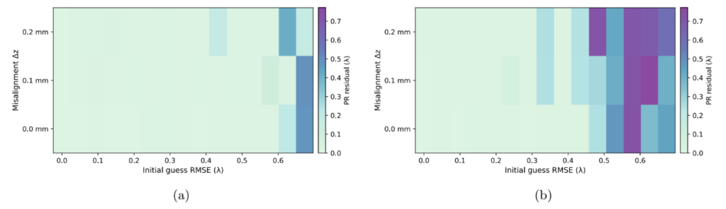
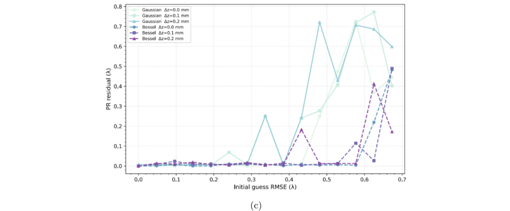
Figure 5: (a) Phase-retrieval results using Bessel-beam illumination for different initial-guess RMSE values from 0 to 0.73λ and axial misalignments from 0 to 0.2 mm. The color represents the residual error after 1000 phase-retrieval iterations. (b) Same as (a), but using Gaussian-beam illumination. (c) Comparison between Bessel-beam and Gaussian-beam illumination under different axial misalignments.
3.1 CNN initial estimator
The CNN forms the first stage of the pipeline. Its role is to estimate the 25 Zernike coefficients directly from a single 512×512 Bessel-beam PSF image. The architecture follows a standard encoder-regression structure and is illustrated in Fig. 8.
The encoder begins with a stem layer consisting of a 5 × 5 convolution with stride 2, followed by a single residual block. This layer increases the channel count from 1 to 32 while reducing the spatial resolution by a factor of two. Four subsequent stages each apply a strided convolution followed by two residual blocks. The channel count doubles in the first three stages (32 → 64 → 128 → 256) and remains fixed in the fourth stage (256 → 256). After five downsampling operations, the feature map has dimensions 256×16×16. Global average pooling then produces a 256-dimensional feature vector, which is mapped to the predicted Zernike coefficients by a three-layer multilayer perceptron (256 → 256 → 128 → 25). GELU activations are used throughout to provide smooth gradients for regression, and Group Normalization with eight groups is used instead of Batch Normalization to avoid unstable normalization statistics at small mini-batch sizes.
The CNN is trained on 10,000 simulated PSF–coefficient pairs generated using the Bessel forward model described in Section 2. Each Zernike coefficient is drawn independently to span the recoverable aberration range.
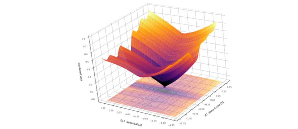
Figure 6: Two-dimensional slice of the phase-retrieval loss surface along the Z7 (horizontal coma) and Z11 (spherical aberration) axes. Multiple local minima are visible even in this restricted projection of the 25-dimensional parameter space.
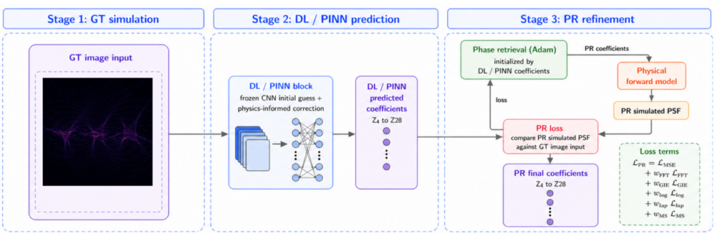
Figure 7: Three-stage hybrid phase-retrieval pipeline. A measured PSF from the test optic serves as the pipeline input. Stage 1 uses the CNN to produce an initial Zernike estimate. Stage 2 uses the physics-informed refinement network to improve that estimate. Stage 3 performs iterative PR using the Adam optimizer.
Training uses the AdamW optimizer with a base learning rate of 2 × 10⁻⁶, a cosine-annealing learning-rate schedule, and a smooth-L1 loss on the predicted coefficient vector,

where ˆck and ck are the predicted and ground-truth values of the k-th Zernike coefficient, K = 25, and $\beta = 0.01$. The smooth-L1 loss behaves like an L1 loss for residuals larger than $\beta$, reducing the influence of outlier coefficients on the gradient. For smaller residuals, it behaves like an L2 loss, supporting stable convergence near the optimum.
The trained CNN was evaluated on a held-out validation set of 300 samples generated from the same forward model. The network achieved a mean coefficient RMSE of 0.1729±0.0526 waves, corresponding to approximately 109 nm at λ = 632 nm. Figure 9 summarizes the per-Zernike error distribution and the corresponding wavefront residual for a representative sample.
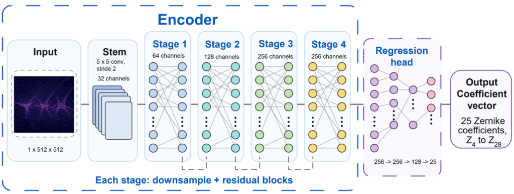
Figure 8: Architecture of the CNN initial estimator. The encoder downsamples the input PSF through a stem and four residual stages, after which global average pooling collapses the spatial dimensions. A three-layer regression head maps the resulting feature vector to the 25 Zernike coefficients Z4 through Z28.
The CNN prediction is sufficient as a coarse estimate but not as a final reconstruction. The systematic residual near the pupil edge indicates that standard coefficient supervision and pixel-space training emphasize the bright central features more strongly than the dim outer rings. Because the outer rings also carry aberration information, the next stage incorporates the optical forward model directly into the loss function.
3.2 Physics-informed refinement network
The CNN is supervised only through the predicted coefficients. It therefore has no direct mechanism for determining whether its prediction, when propagated through the optical system, reproduces the measured PSF. A coefficient vector can be close to the ground truth while still producing a visibly different irradiance pattern, especially in dim PSF regions. The physics-informed refinement network (PINN) closes this loop by incorporating the differentiable forward model into the training loss. The architecture is shown in Fig. 10.
The PINN consists of three components. The first is a frozen copy of the CNN initial estimator, with all parameters held fixed during PINN training. This frozen CNN provides a stable baseline from which the refinement network learns corrections. The second component is the Fresnel-propagation forward model from Section 2, implemented using fast Fourier transforms, complex-exponential phase multiplications, and pointwise operations. Because each propagation step is differentiable, gradients can pass through the renderer during backpropagation, even though the renderer contains no learnable parameters. This structure makes the network physics-informed: the loss can be evaluated on the rendered irradiance, forcing the predicted coefficients to reproduce the measured PSF through the optical model.
The third component is the refinement network, denoted RefineDeltaCNN. It is a smaller convolutional encoder than the initial estimator, with three downsampling stages instead of four and a base channel width of 24 rather than 32. Its input is a three-channel tensor formed by stacking the measured PSF, the coarse simulated PSF rendered from the frozen CNN prediction, and their pointwise residual. The residual channel is the key physics-informed feature because it identifies where the forward simulation disagrees with the measurement. The refinement encoder outputs a 25-dimensional correction vector $\Delta c$, which is clipped to [−0.5, 0.5] waves per coefficient to prevent unphysically large updates. The refined coefficient vector is $c = c_0 + \Delta c$, where $c_0$ is the frozen CNN prediction.
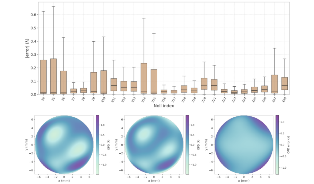
Figure 9: Validation results of the CNN initial estimator on 300 held-out samples. Top: per-Zernike absolute-error distribution, with each box summarizing the error of one coefficient over the validation set. Bottom: ground-truth map (left), CNN model result (center), and residual error (right), shown together as a representative wavefront residual map. The largest residuals are concentrated near the pupil edge, where the dim outer Bessel rings carry less information per pixel and contribute less to the standard mean-squared error during training.
The PINN is trained with a composite loss that combines coefficient supervision, image-domain supervision, and a small regularization term on the correction magnitude:

The four image-domain terms apply mean-squared error and log-domain mean-squared error to both the coarse PSF Icoarse and the final PSF Ifinal. The coefficient term Lcoef is the smooth-L1 loss defined in Eq. 2, applied to the refined coefficient vector c. The pixel-space mean-squared-error term is:

where I (·) denotes either Icoarse or Ifinal, Imeas is the measured PSF, and N is the number of pixels in the region of interest. The log-domain term is:

where ε is a small positive constant used to avoid numerical instability in the logarithm. Taking the logarithm before computing the squared error increases the contribution of dim PSF regions, which would otherwise be dominated by the bright central peak under Eq. 4. This term directly addresses the systematic edge residual observed in the CNN-only result.
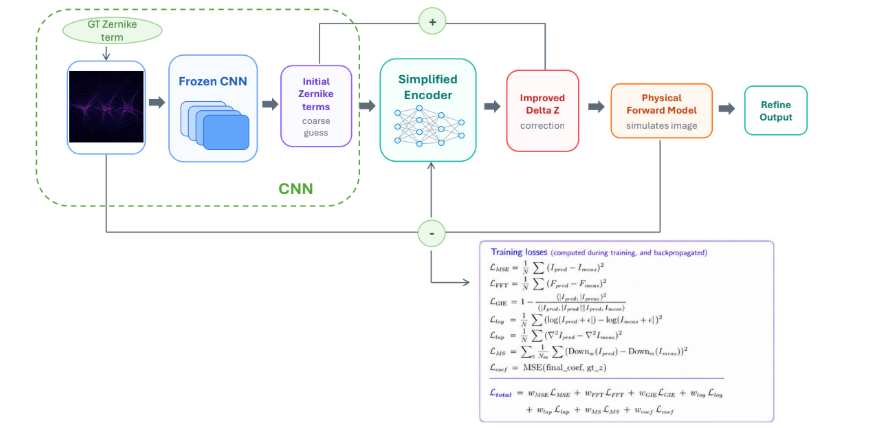
Figure 10: Architecture of the physics-informed refinement network. A frozen copy of the CNN initial estimator produces an initial Zernike vector c0, which is rendered through the differentiable Fresnel forward model to produce a coarse simulated PSF Icoarse. The measured PSF Imeas, the coarse simulated PSF, and their residual Imeas − Icoarse are stacked as a three-channel input to a smaller refinement encoder, which predicts a coefficient correction ∆c. The refined coefficients c0 + ∆c are rendered again to produce the final simulated PSF Ifinal. Both renderings are compared with the measured PSF, and the refined coefficients are compared with the ground truth, in a composite training loss.
The correction-magnitude regularizer is:

which discourages unnecessarily large coefficient updates. The image-domain weights are wC = 0.2, wF = 1.0, wlC = 0.02, and wlF = 0.05. The final-rendering terms are weighted more strongly because they correspond to the refined prediction. The global image-domain weight is wimg = 10, the coefficient weight is wcoef = 1.0, and the correction-magnitude weight is w∆ = 10−4
The PINN is trained from scratch while using the frozen CNN to provide the initial estimate at each iteration. The same forward model is used during training and inference, avoiding a mismatch between the training renderer and the inference pipeline. Evaluated on the same 300-sample validation set used in Section 3.1, the PINN achieved a mean coefficient RMSE of 0.1056 ± 0.0334 waves, corresponding to approximately 67 nm at λ = 632 nm as shown in Fig. 11. This represents a 38.9% reduction in residual error relative to the CNN-only baseline. As shown in Fig. 12, the PINN reduces the per-Zernike coefficient error and suppresses the wavefront residual compared with the CNN-only result. The systematic edge residual observed in the CNN reconstruction is substantially reduced, consistent with the role of the log-domain image loss in increasing the contribution of dim outer-ring regions.
The PINN places the predicted coefficient vector sufficiently close to the global minimum of the optical forward model for classical gradient-based PR to be applied. In the full pipeline, the PINN therefore serves not as the final reconstruction, but as a physics-consistent warm start for the iterative refinement stage.
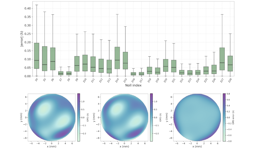
Figure 11: Validation results of the PINN on the same 300-sample held-out set used to evaluate the CNN. Top: per-Zernike absolute-error distribution. Bottom: ground-truth map (left), PINN model result (center), and residual error (right). Compared with the PINN result in Fig. 9, the per-Zernike error distributions are tighter and the wavefront residual at the pupil edge is visibly reduced.
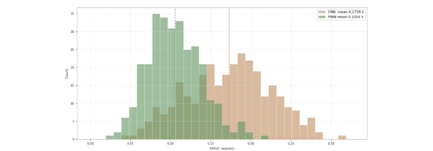
Figure 12: Comparison of CNN-only and PINN-refined reconstruction results. The PINN reduces the residual error by 38.9% relative to the CNN-only baseline and suppresses the systematic edge residual in the reconstructed wavefront.
3.3 Iterative phase retrieval refinement
The PINN prediction is used as the initialization for the final iterative phase-retrieval stage. At this stage, no ground-truth coefficients are used. The optimization minimizes the discrepancy between the measured PSF and a rerendered PSF computed from the current coefficient estimate using the same Fresnel forward model. The optimizer is Adam:

where c(t) is the coefficient vector at iteration t, and $\nabla_c L_{\text{PR}}$ is the gradient of the phase-retrieval objective with respect to c.
The phase-retrieval objective combines six complementary loss terms, each measuring a different aspect of the discrepancy between predicted and measured irradiance patterns:

This combination is used because no single image-similarity metric captures all relevant features of a Bessel-beam PSF. Combining pixel-domain, frequency-domain, and gradient-domain terms provides a richer optimization signal and reduces sensitivity to spurious local minima. Two terms are written explicitly below; the remaining terms follow standard forms from image reconstruction and are summarized in Table 1.
The first term is an intensity-weighted pixel-space mean-squared error:

where p = 4, and the angle brackets denote a spatial mean. This weighting concentrates the gradient on bright structural features, where small coefficient errors produce large intensity changes, while reducing the influence of sampling noise in dim regions. The second term is the Fourier-domain loss:

where $\mathcal{F}$ denotes the two-dimensional discrete Fourier transform, and M(u) is a circular low-pass mask. The mask excludes the highest spatial frequencies, where the scaled-Fresnel rendering pipeline can introduce sampling artifacts that should not contribute to the loss. The logarithm compresses the dynamic range of the Fourier magnitude, allowing low-amplitude frequency components to contribute to the gradient.
The remaining four terms, the log-domain pixel loss $L_{\text{log}}$, normalized correlation loss $L_{\text{GIE}}$, Laplacian loss $L_{\text{Lap}}$, and multiscale average-pooling loss $L_{\text{MS}}$, follow standard forms from image reconstruction. Their definitions, weights, and roles are summarized in Table 1. The log-domain pixel loss has the same form as Eq. 5 and is included to increase sensitivity to dim outer-ring regions.
The pooling scales $s \in {2, 7}$ in $L_{\text{MS}}$ span the characteristic pixel widths of the bright Bessel core and the first few outer rings. The loss weights in Table 1 were tuned empirically to balance terms with different numerical scales. The optimizer is run for 800 iterations starting from the PINN prediction, with gradient-norm clipping at 20. A backtracking rule adjusts the learning rate to 0.97 and restores the best-so-far coefficients after six iterations without improvement.
Evaluated over 100 noise-free test cases, the full pipeline achieved a final coefficient RMSE of 0.0022±0.0056 waves, corresponding to approximately 1.4 nm RMS at λ = 632 nm. Figure 13 shows the per-Zernike error distribution after the full three-stage pipeline. The per-coefficient errors are in the single-thousandths-of-a-wave range across nearly all 25 modes. The residual wavefront map is essentially flat over the pupil interior, with the small remaining structure concentrated near the pupil edge.
This result represents the performance ceiling under noise-free conditions. Quantifying the impact of measurement noise on the achievable accuracy is left to future work.
| Term | Form | Role | Weight |
|---|---|---|---|
| $L_{\text{MSE}}$ | Intensity-weighted pixel MSE, Eq. 9 | Bright-feature agreement | 1 |
| $L_{\text{FFT}}$ | Log-magnitude masked Fourier MSE, Eq. 10 | Periodic ring-spacing agreement | 2 |
| $L_{\text{log}}$ | $\text{MSE}\left(\log(I_{\text{pred}} + \varepsilon), \log(I_{\text{meas}} + \varepsilon)\right)$ | Dim outer-ring agreement | $10^{-10}$ |
| $L_{\text{GIE}}$ | $1 – \frac{\langle I_{\text{pred}}, I_{\text{meas}} \rangle^2}{\ | I_{\text{pred}}\ | _2^2 \ |
| $L_{\text{Lap}}$ | $\text{MSE}\left(\nabla^2 I_{\text{pred}}, \nabla^2 I_{\text{meas}}\right)$ | Edge-sharpness agreement | $10^2$ |
| $L_{\text{MS}}$ | $\sum_{s \in {2,7}} \text{MSE}\left(\text{Down}s I{\text{pred}}, \text{Down}s I{\text{meas}}\right)$ | Multiscale structural agreement | 10 |
Table 1: Summary of the six phase-retrieval loss terms in Eq. 8. Indices r and u denote spatial and spatial-frequency coordinates, respectively, and N is the number of samples in the relevant domain. The angle brackets in the inner-product expressions denote spatial sums.
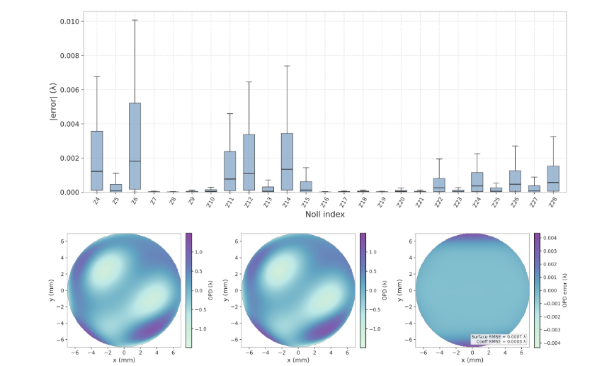
Figure 13: Validation results of the full three-stage pipeline, evaluated on 100 noise-free test cases. Top: per-Zernike absolute-error distribution, with the vertical scale in the single-thousandths-of-a-wave range. Bottom: ground-truth map (left), full pipeline result (center), and residual error (right). Compared with the PINN result in Fig. 11, the residual is essentially flat over the pupil interior, with only a thin band of residual structure remaining at the pupil edge. Surface RMSE = 0.0007, Coeff RMSE = 0.0003.
4. CONCLUSION
In conclusion, we proposed a proof-of-concept phase-retrieval framework that extends the recoverable dynamic range at both the physical and algorithmic levels. At the physical level, Bessel-beam illumination was used to preserve aberration-dependent phase information within the measured irradiance distribution over an extended propagation distance. Compared with Gaussian-beam illumination, the Bessel-beam PSF retains distinguishable structural features over a longer axial range, providing a more robust physical encoding of the wavefront.
At the algorithmic level, we developed a three-stage hybrid refinement pipeline that combines a CNN initial estimator, a physics-informed refinement network, and iterative PR with a multidimensional loss function. The presented simulation case used a single-mode fiber source incident on an axicon grating with a cone angle of 0.0458 rad. A 4 lp/mm linear grating generated three Bessel-beam orders, and the observation plane was located 457 mm from the phase map. Under this configuration, the CNN achieved a coefficient RMSE of 0.1729±0.0526 waves, which was reduced to 0.1056 ± 0.0334 waves by the physics-informed refinement network. After final iterative PR, the coefficient RMSE was further reduced to 0.0022±0.0056 waves, corresponding to approximately 1.4 nm RMS at λ = 632 nm. The method was demonstrated for wavefronts with a maximum peak-to-valley value of 7.3λ.
These simulation results indicate that Bessel-beam-based PR is a promising approach for extending the practical capture range of wavefront reconstruction. Because the recovered phase is no longer restricted to strongly converging wavefronts near focus, the method can also be applied to near-plane-wave and, within a certain range, divergent wavefront conditions. This property expands the flexibility of PR for practical optical-system configurations.
Although this work focuses on Bessel-beam illumination, the hybrid reconstruction pipeline is not limited to Bessel beams. The same CNN, physics-informed refinement, and iterative-optimization strategy can also be applied to Gaussian-beam-based PR, although with a smaller recoverable dynamic range because of the reduced axial persistence of the Gaussian-beam irradiance structure. More broadly, the proposed framework suggests a pathway toward flexible wavefront sensing for biomedical imaging, optical metrology, and adaptive optical characterization.
Acknowledgments
The authors acknowledge the use of AI-based tools for grammar checking and language polishing during manuscript preparation. Figures 7, 8, and 10 were generated with assistance from AI-based tools and were reviewed and edited by the authors for scientific accuracy and consistency with the described methods.
Disclosures
The authors declare no conflicts of interest.
REFERENCES
- Fienup, J. R., “Phase retrieval algorithms: a comparison,” Applied Optics 21(15), 2758–2769 (1982).
- Jagatap, G. and Hegde, C., “Phase retrieval using untrained neural network priors,” in Workshop on Solving Inverse Problems with Deep Networks, Proceedings of the 33rd Conference on Neural Information Processing Systems, OpenReview.net (2019).
- Zhou, Z., Zhang, J., Fu, Q., and Nie, Y., “Phase-diversity wavefront sensing enhanced by a fourier-based neural network,” Optics Express 30(19), 34396–34410 (2022).
- Paxman, R. G., Schulz, T. J., and Fienup, J. R., “Joint estimation of object and aberrations by using phase diversity,” Journal of the Optical Society of America A 9(7), 1072–1085 (1992).
- Durnin, J., “Exact solutions for nondiffracting beams. i. the scalar theory,” Journal of the Optical Society of America A 4(4), 651–654 (1987).
- McGloin, D. and Dholakia, K., “Bessel beams: diffraction in a new light,” Contemporary Physics 46(1), 15–28 (2005).
- Lee, K.-S. and Rolland, J. P., “Bessel beam spectral-domain high-resolution optical coherence tomography with micro-optic axicon providing extended focusing range,” Optics Letters 33(15), 1696–1698 (2008).
- Jin, K. H., McCann, M. T., Froustey, E., and Unser, M., “Deep convolutional neural network for inverse problems in imaging,” IEEE Transactions on Image Processing 26(9), 4509–4522 (2017).
- Rivenson, Y., Zhang, Y., Günaydın, H., Teng, D., and Ozcan, A., “Phase recovery and holographic image reconstruction using deep learning in neural networks,” Light: Science & Applications 7, 17141 (2018).
- Khonina, S. N., Kazanskiy, N. L., Karpeev, S. V., and Butt, M. A., “Bessel beam: Significance and applications—a progressive review,” Micromachines 11(11), 997 (2020).
- Birch, P., Ituen, I., Young, R., and Chatwin, C., “Long-distance bessel beam propagation through kolmogorov turbulence,” Journal of the Optical Society of America A 32(11), 2066–2073 (2015).
- Chen, Z., Parks, R. E., Dhawan, B., Gurunarayanan, S. P., and Kim, D., “Quasi-ray tracing realization using a bessel beam for optical alignment,” Optics Express 32(27), 48571–48582 (2024).
- LeCun, Y., Boser, B., Denker, J. S., Henderson, D., Howard, R. E., Hubbard, W., and Jackel, L. D., “Backpropagation applied to handwritten zip code recognition,” Neural computation 1(4), 541–551 (1989).
- Kingma, D. P. and Ba, J., “Adam: A method for stochastic optimization,” in Proceedings of the 3rd International Conference on Learning Representations (ICLR), (2015).
- Jiang, L., Dai, B., Wu, W., and Loy, C. C., “Focal frequency loss for image reconstruction and synthesis,” in Proceedings of the IEEE/CVF International Conference on Computer Vision (ICCV), 13919–13929 (2021).
- Eilertsen, G., Kronander, J., Denes, G., Mantiuk, R. K., and Unger, J., “HDR image reconstruction from a single exposure using deep CNNs,” ACM Transactions on Graphics 36(6), 178:1–178:15 (2017).
- Li, S., Xu, X., Nie, L., and Chua, T.-S., “Laplacian-steered neural style transfer,” in Proceedings of the 25th ACM International Conference on Multimedia (MM ’17), 1716–1724 (2017).
- Wang, Z., Simoncelli, E. P., and Bovik, A. C., “Multiscale structural similarity for image quality assessment,” in The Thirty-Seventh Asilomar Conference on Signals, Systems and Computers, 2, 1398–1402 (2003).